Theorem 7.10: The following equivalence holds for all square matrices $\mx{A}$,
\begin{equation}
\begin{array}{ll}
(i) & \spc\text{The column vectors of}\spc \mx{A} \spc\text{is a basis} \\
(ii) & \spc\text{The row vectors of}\spc \mx{A} \spc\text{is a basis} \\
(iii) & \spc\text{The matrix equation} \spc \mx{A} \vc{x} = 0 \spc\text{has only one solution} \spc \vc{x}=0 \\
(iv) & \spc\text{The matrix equation}\spc \mx{A} \vc{x} = \vc{y} \spc\text{has a solution for every} \spc \vc{y} \\
(v) & \spc\text{The matrix} \spc \mx{A} \spc\text{is invertible} \\
(vi) & \spc\det \mx{A} \neq 0 \\
\end{array}
\end{equation}
Theorem 10.3: A matrix $\mx{A}$ is diagonalizable if and only if there exists a basis of eigenvectors. Furthermore, in the factorization
$ \mx{A} = \mx{V} \mx{D} \mx{V}^{-1}$, the columns of $\mx{V}$ correspond to eigenvectors and the corresponding elements of the diagonal matrix $\mx{D}$ are the eigenvalues.
Theorem 10.4: If the $n \times n$ matrix $\mx{A}$ has $n$ different eigenvalues, then $\mx{A}$ is diagonalizable. Furthermore, $n$ eigenvectors corresponding to different eigenvalues are always linearly independent.
Theorem 10.8: For symmetric matrix $\mx{A}$, it is possible to find an orthogonal matrix $\mx{U}$ and diagonal matrix $\mx{D}$ such that
\begin{equation}
\mx{A} = \mx{U} \mx{D} \mx{U}^{-1} = \mx{U} \mx{D} \mx{U}^{T} .
\end{equation}
In other words, it is possible to diagonalise using an orthonormal basis of eigenvectors.
Theorem 10.7: The eigenvalues of a symmetric matrix $\mx{A}$ are all real.
Theorem 10.9: Definiteness and eigenvalues A symmetric real $n \times n$ matrix $\mx{A}$ is
\begin{align}
\begin{array}{ll}
&(1) & \text{positive definite if and only if all eigenvalues are positive} \\
&(2) & \text{positive semi-definite if and only if all eigenvalues are non-negative} \\
&(3) & \text{negative definite if and only if all eigenvalues are negative} \\
&(4) & \text{negative semi-definite if and only if all eigenvalues are non-positive} \\
&(5) & \text{indefinite if and only if there are both positive and negative eigenvalues} \\
\end{array}
\end{align}
Theorem 8.8: Dimension Theorem For an $m\times n$ matrix $\mx{A}$, i.e., with $n$ columns, it holds that
\begin{equation}
\rank(\mx{A}) + \nullity(\mx{A}) = n.
\end{equation}
Theorem 8.9: The rank of a matrix $\mx{A}$ (of size $m\times n$) is the largest integer $r$ for
which some $r\times r$-minor is $\neq 0$.
Definition 10.4: A matrix $\mx{A}$ is diagonalizable, if there exists an invertible matrix $\mx{V}$ and a diagonal matrix $\mx{D}$ such that
\begin{equation}
\mx{A} = \mx{V} \mx{D} \mx{V}^{-1} .
\end{equation}
In this chapter, we introduce the concepts of eigenvalues and eigenvectors of a square matrix. These concepts have numerous uses, for example, to better understand and visualize linear mappings, to understand the stability of mechanical constructions, for solving systems of differential equations, to recognize images, to interpret and visualize quadratic equations, and for image segmentation. First, let us start with two examples.
Example 10.1:Eigenfaces
There are many methods for recognizing faces in images. State of the art methods typically use deep learning, for which linear algebra is an important part. One popular approach for understanding and compressing face images is to use, so called, eigenfaces. This is illustrated in Interactive Illustration 10.1, where we show an example of how new faces can be generated using two parameters. By just specifying two numbers, it is possible to synthesize a whole range of images as is shown in the figure. Thus the technique can be used for synthesizing new images. This can also bee seen as image compression since only two numbers need to be stored for every new image. The technique can also be used for
image understanding in the following way. For new images one may calculate what the corresponding coordinates $(x_1,x_2)$ are. Different regions in $R^2$ correspond to smiling face, open mouth etc.
Interactive Illustration 10.1:
Left: two coordinates $(x_1,x_2)$ specify input. Right: the result of the mapping $(x_1,x_2) \mapsto \vc{O} + x_1 \vc{E}_1 + x_2 \vc{E}_2$,
where $\vc{O}$ is the mean image and $\vc{E}_1$ and $\vc{E}_2$ are the first two eigenfaces. Try moving the black circle and see how the output changes.
Interactive Illustration 10.1:
Left: two coordinates $\hid{(x_1,x_2)}$ specify input. Right: the result of the mapping $\hid{(x_1,x_2) \mapsto \vc{O} + x_1 \vc{E}_1 + x_2 \vc{E}_2}$,
where $\hid{\vc{O}}$ is the mean image and $\hid{\vc{E}_1}$ and $\hid{\vc{E}_2}$ are the first two eigenfaces. Try moving the black circle and see how the output changes.
The mean image, $\vc{O}$, and the two eigenfaces, $\vc{E}_1$ and $\vc{E}_2$, are shown below.
The images used to generated $\vc{O}$, $\vc{E}_1$, and $\vc{E}_2$ are shown in Figure 10.2. This process is explained later in a bit more detail in Example 10.18 once we have learnt more about eigenvalues and eigenvectors. Briefly, one can say that the images in Figure 10.2 are used to calculate the mean $O$ and the covariance matrix. The two eigenvectors of the covariance matrix corresponding to the two largest eigenvalues are used as $\vc{E}_1$ and $\vc{E}_2$.
Interactive Illustration 10.2:
These 23 images were used in computing the basis used in Interactive Illustration 10.1.
Interactive Illustration 10.2:
These 23 images were used in computing the basis used in \linkref{Interactive Illustration}{fig_eigenfaces}.
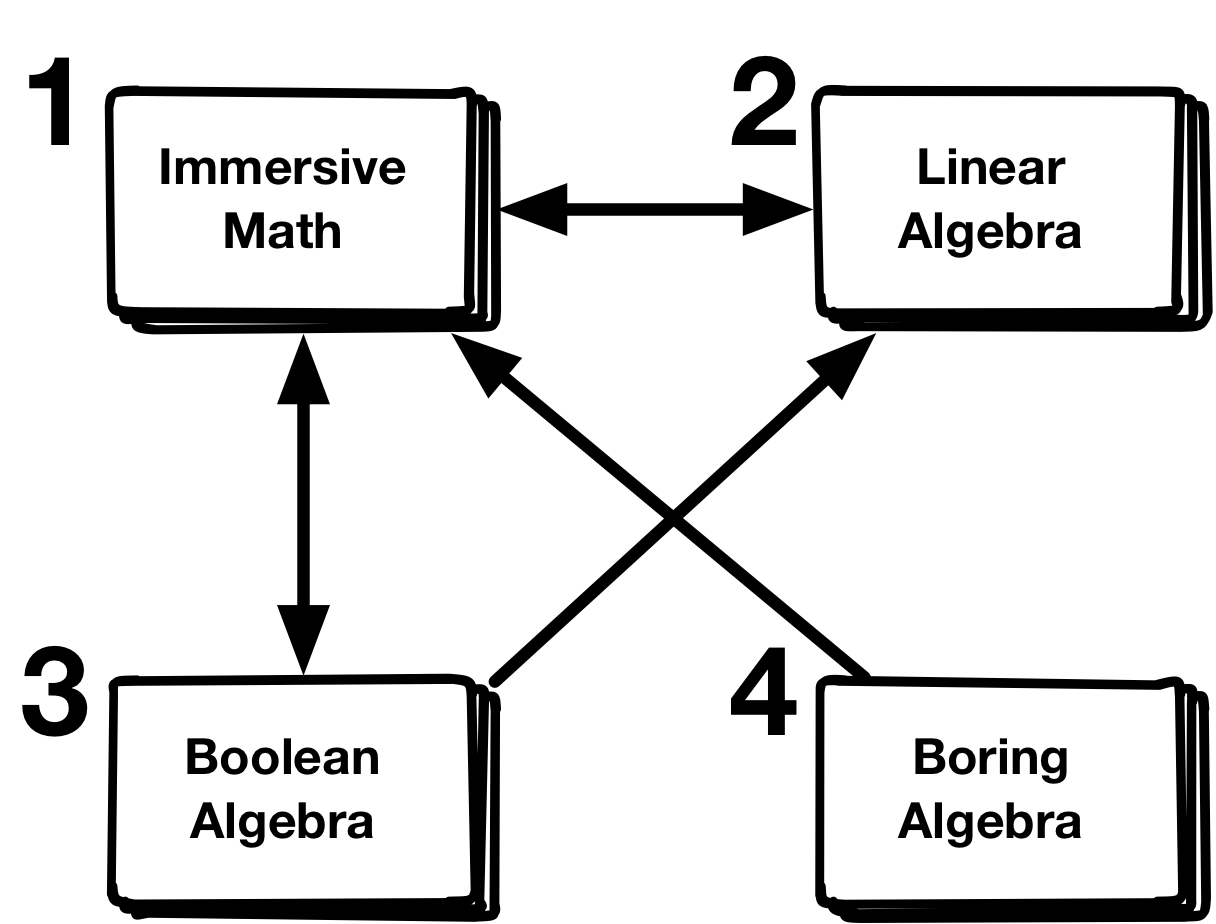
Example 10.2:Pagerank How does Google rank web pages?
In this example, we will look at a simplified model for ranking web pages. The main idea is that a web page has a higher rank if many pages (with high rank) links to this page. The problem is recursive. In order to calculate the rank of one page, you need to know the ranks of the other pages. Another way to look at this is to think of a person that randomly clicks on one of the links of a homepage. After random browsing, the page rank is the probability that you are on a certain homepage. In order to connect all homepages one has the idea that with a small probability (say 15 percent) one jumps to a totally random homepage. Let's look at a toy example.
Assume that there are four homepages on the internet, 1 - 'Immersive Math', 2 - 'Linear Algebra', 3 - 'Boolean Algebra' and 4 - 'Boring Algebra'.
The links from one homepage to another are illustrated as arrows in the figure.
Assume that the probability of being at a homepage is given by a vector $\vc{v} = \begin{pmatrix} v_1 \\ v_2 \\ v_3 \\ v_4 \end{pmatrix}$, where $v_i$ is the probability of being at homepage with number $i$. If you choose randomly among the links of one homepage, the probability of being on a homepage becomes $ \vc{w} = \mx{A} \vc{v}$,
where the transition matrix, $\mx{A}$, is
The first column has two entries. If you are at homepage $1$ there are two links, one to page 2 and one to page 3. There is thus a probability $0.5$ of ending up in homepage 2 and probability $0.5$ of ending up in homepage 3. Similarly, the entries in column $j$ depend on what links there are on homepage $j$.
For the page rank problem, one usually modifies the probability in the following way. You have a small probability, say $0.15$, that you choose a random homepage with equal probability and then a probability $0.85$ that you choose the next homepage according to the links. The transition matrix becomes
This is a linear equation in the unknowns $\vc{p}$, which could be calculated using Gaussian elimination, but it is also connected to the concept of eigenvectors that we are discussing in this chapter.
In this example, the vector $\vc{p}$ is
So obviously 'Immersive Math' should be the top choice.
A continued discussion on how to solve the pagerank problem for really large networks (like the internet) will be given in Example 10.12 using what we will learn about eigenvalues and eigenvectors in this chapter.
Let us start with the definition of eigenvalues and eigenvectors.
Definition 10.1:Eigenvalue and Eigenvector
Let $\mx{A}$ be a square matrix. A non-zero column vector $\vc{v}$
is called an eigenvector if $\mx{A}\vc{v}$ is parallell to $\vc{v}$, i.e., if there exists a scalar $\lambda$ such that
The scalar $\lambda$ is then called an eigenvalue.
In Chapter 9, we saw that a linear mapping can be represented as matrix multiplication. For linear mappings, we define eigenvectors and eigenvalues in the corresponding way, i.e., for a linear mapping $F$, we say that a non-zero vector $\vc{v}$ is an eigenvector if $F(\vc{v})$ is parallel to $\vc{v}$. This means that $F(\vc{v}) = \lambda \vc{v}$. In the same way, $\lambda$ is called the eigenvalue.
Example 10.3:Find The Eigenvector Game
Notice that eigenvectors for linear mappings or transformations are well defined without knowing the coordinate system. We illustrate the basic concept in the following example and interactive illustration, which can be thought of as a game 'Find the Eigenvectors'.
$\vc{v}$
$F(\vc{v})$
$\vc{e}_1$
$\vc{e}_2$
$\frac{\ln{F(\vc{v})}}{\ln{\vc{v}}}=$
Interactive Illustration 10.3:
An example of a mapping from $\vc{v}$ (red vector) to $F(\vc{v})$ (blue vector).
The unknown linear mapping $F$ takes a two-dimensional vector $\vc{v}$ and returns a two-dimensional vector $F(\vc{v})$. In the illustration, you may move the input vector $\vc{v}$ and can observe the result. Try to change $\vc{v}$ until $F(\vc{v})$ and $\vc{v}$ are parallel. When this occurs, you have found an eigenvector.
Interactive Illustration 10.3:
An example of a mapping from $\hid{\vc{v}}$ (red vector) to $\hid{F(\vc{v})}$ (blue vector).
The unknown linear mapping $\hid{F}$ takes a two-dimensional vector $\hid{\vc{v}}$ and returns a two-dimensional vector $\hid{F(\vc{v})}$. In the illustration, you may move the input vector $\hid{\vc{v}}$ and can observe the result. Try to change $\hid{\vc{v}}$ until $\hid{F(\vc{v})}$ and $\hid{\vc{v}}$ are parallel. When this occurs, you have found an eigenvector.
In Interactive Illustration 10.3,
we also calculate $\frac{\ln{ F(\vc{v}) } }{\ln{\vc{v}}}$.
Try to see how many eigenvectors you can find by interactively moving the input vector ${\vc{v}}$ and attempt to determine the eigenvalue to each eigenvector.
In Interactive Illustration 10.3,
you may have noticed that changing the length of the vector $\vc{v}$ does not change the fact that it is (or is not) an eigenvector. This follows from the linearity of the mapping, which is described in the following theorem.
Theorem 10.1:
If $\vc{v}$ is an eigenvector with eigenvalue $\lambda$, then $\mu \vc{v}$ is also an eigenvector with the same eigenvalue for each $\mu \neq 0$.
If $\vc{v}$ is an eigenvector with eigenvalue $\lambda$, then $\vc{v} \neq 0$ and
$F(\vc{v}) = \lambda \vc{v}$. For each non-zero multiple $\vc{u} = \mu \vc{v}$, we have that $\vc{u} \neq 0$ and that
$F(\vc{u}) = F( \mu \vc{v}) = \mu F(\vc{v}) = \mu \lambda \vc{v} = \lambda \vc{u}$. This proves the theorem.
$\square$
So the eigenvectors can always be rescaled. However, remember that eigenvectors have to be non-zero.
Example 10.4:Maximum Elongation of Linear Functions
In the Example 10.3, we illustrated eigenvectors and eigenvalues interactively. One interesting question is to study how much larger the output $F(\vc{v})$ of a linear mapping $F$ is in relation to its input vector $\vc{v}$. In the figure below, we keep the length of the input vector $\vc{v}$ to one. You may rotate the input vector using the slider below the figure. Notice that the tip of the output vector $F(\vc{v})$ lies on an ellipse. There is one direction which gives the largest elongation and perpendicular to this direction are the input vectors that gives the smallest elongation. Later in this chapter (in Section 10.6), we will see why this is so and how these directions can be calculated.
$\vc{v}$
$F(\vc{v})$
$\vc{e}_1$
$\vc{e}_2$
Interactive Illustration 10.4:
An example of a mapping from $\vc{v}$ (red vector) to $F(\vc{v})$ (blue vector). The length of the input vector is fixed to one. Can you find the input vector $\vc{v}$ that gives the longest output vector $F(\vc{v})$. Try a bit first and then click on forward to see the ellipse of possible output vector endpoints.
Interactive Illustration 10.4:
An example of a mapping from $\hid{\vc{v}}$ (red vector) to $\hid{F(\vc{v})}$ (blue vector). The length of the input vector is fixed to one. Can you find the input vector $\hid{\vc{v}}$ that gives the longest output vector $\hid{F(\vc{v})}$. Try a bit first and then click on forward to see the ellipse of possible output vector endpoints.
In this section, we will describe how eigenvectors and eigenvalues can be calculated. (Note: The methods is based on finding roots to a polynomial. In practice, there are more efficient numerical methods for finding eigenvalues and eigenvectors. The connection between eigenvalues and roots are then used to calculate roots using eigenvalues and not the other way around).
Definition 10.2:Characteristic Polynomial
Let $\mx{A}$ be a square matrix of size $n \times n$. The polynomial
\begin{equation}
p_{\mx{A}}(\lambda) = \det(\lambda I - \mx{A})
\end{equation}
(10.6)
is then called the characteristic polynomial.
Theorem 10.2:
The characteristic polynomial is a polynomial of degree $n$ in $\lambda$.
The eigenvalues $\lambda$ to the matrix $\mx{A}$ are the roots of the characteristic polynomial $p_{\mx{A}}(\lambda)$.
If $\vc{v}$ is an eigenvector, then the matrix $(\lambda I - \mx{A})$ has a non-zero null vector. According to
Theorem 7.10, this means that $p_{\mx{A}}(\lambda) = \det( \lambda I - \mx{A} ) = 0$.
This proves that the eigenvalues are roots of the characteristic polynomial. Vice versa, for every root $\lambda$ of the characteristic polynomial, the equation $( \lambda I - \mx{A} ) \vc{v} = 0$ has a non-zero solution $\vc{v}$. This gives an eigenvector, since $\mx{A}\vc{v} = \lambda \vc{v}$.
$\square$
Example 10.5:Calculating Eigenvalues and Eigenvectors using the Characteristic Polynomial Calculate the eigenvalues and eigenvectors of
The two eigenvalues are thus $\lambda_1 = 1$ and $\lambda_2 = 3/2$.
For each eigenvalue, the corresponding eigenvectors can be found by solving
$( \lambda I - \mx{A} ) \vc{v} = 0$.
This system of equations has the parametric solution
\begin{equation}
\vc{v} = t \begin{pmatrix}
3\\
4
\end{pmatrix} .
\end{equation}
(10.16)
Thus all vectors
\begin{equation}
\vc{v} = t \begin{pmatrix}
3\\
4
\end{pmatrix} , \quad t \neq 0
\end{equation}
(10.17)
are eigenvectors corresponding to eigenvalue $3/2$.
Interactive Illustration 10.5 shows this linear mapping. By moving the red input arrow, it is possible to visually "prove" that these vectors are indeed eigenvectors since the blue output vector becomes parallel with the red input vector.
$\vc{v}$
$F(\vc{v})$
Interactive Illustration 10.5:
In this interactive illustration, the linear mapping $F(\vc{v}) = \mx{A}\vc{v}$ is illustrated, where the input vector $\vc{v}$ is drawn in red and the output vector $F(\vc{v})$ is drawn in blue. By putting the input vector in $(1, 2)$ it is possible to verify that this is indeed an eigenvector by noticing that the blue output vector $F(\vc{v})$ is parallel with the input vector. One can also verify that the eigenvector is $1$ since the blue vector is exactly as long as the red one. It is possible to do a similar check for the eigenvector in $(3,4)$. Note how the two eigenvectors are very close to each other in in this example, since one is found at $(2,4)$ and the other at $(3,4)$. However, the eigenvector at $(3,4)$ has a larger eigenvalue ($3/2$ instead of $1$) so the blue vector grows considerably when moving from $(2, 4)$ to $(3,4)$.
Interactive Illustration 10.5:
In this interactive illustration, the linear mapping $\hid{F(\vc{v}) = \mx{A}\vc{v}}$ is illustrated, where the input vector $\hid{\vc{v}}$ is drawn in red and the output vector $\hid{F(\vc{v})}$ is drawn in blue. By putting the input vector in $\hid{(1, 2)}$ it is possible to verify that this is indeed an eigenvector by noticing that the blue output vector $\hid{F(\vc{v})}$ is parallel with the input vector. One can also verify that the eigenvector is $\hid{1}$ since the blue vector is exactly as long as the red one. It is possible to do a similar check for the eigenvector in $\hid{(3,4)}$. Note how the two eigenvectors are very close to each other in in this example, since one is found at $\hid{(2,4)}$ and the other at $\hid{(3,4)}$. However, the eigenvector at $\hid{(3,4)}$ has a larger eigenvalue ($\hid{3/2}$ instead of $\hid{1}$) so the blue vector grows considerably when moving from $\hid{(2, 4)}$ to $\hid{(3,4)}$.
Eigenvectors and eigenvalues are connected to a concept of diagonalization.
The idea here is that a linear mapping is particularly simple if one chooses the eigenvectors as basis vectors. We will need a definition of diagonalization for both a linear mapping and for a matrix. These two definitions are essentially the same.
For the first definition, we should remember that a linear mapping $F(\vc{v})$ can be defined even without a basis. An example is the linear mapping where the output vector is just the input vector but twice as long - this can be understood regardless of the basis chosen. However, if we do select a basis for the linear mapping, we can write the linear mapping on the form $F(\vc{v}) = \mx{A}\vc{v}$, where $\mx{A}$ is called the transformation matrix. The transformation matrix depends on the basis chosen. With this refresher in mind we are now ready for the definition of diagonalizability for a linear mapping.
Definition 10.3:
A linear mapping $F$ is diagonalizable if there is a basis, such that the transformation matrix is a diagonal matrix.
Definition 10.4:
A matrix $\mx{A}$ is diagonalizable, if there exists an invertible matrix $\mx{V}$ and a diagonal matrix $\mx{D}$ such that
The matrix $\mx{A}$ is factorized as a product of three matrices $\mx{V}$, $\mx{D}$, and
$\mx{V}^{-1}$. Such factorizations are extremely useful in many applications. We will give a few such applications later in this chapter.
To understand how diagonalization relates to eigenvectors and eigenvalues, we rearrange the matrix equation as
Let the column vectors of $\mx{V}$ be $(\vc{v}_1, \ldots, \vc{v}_n)$ and let the diagonal elements of $\mx{D}$ be $(\lambda_1, \ldots, \lambda_n)$.
Using this notation, the equation can be written
so the columns of $\mx{V}$ are eigenvectors to $\mx{A}$ and the corresponding eigenvalue is found at the corresponding diagonal element of $\mx{D}$.
This can be summarized in a theorem.
Theorem 10.3:
A matrix $\mx{A}$ is diagonalizable if and only if there exists a basis of eigenvectors. Furthermore, in the factorization
$ \mx{A} = \mx{V} \mx{D} \mx{V}^{-1}$, the columns of $\mx{V}$ correspond to eigenvectors and the corresponding elements of the diagonal matrix $\mx{D}$ are the eigenvalues.
Example 10.6:Single Roots and Diagonalizable Matrices Check if the matrix
For matrices of size $2 \times 2$, the characteristic polynomial is of degree 2 and there are therefore 2 roots (if you count complex roots and take multiplicity of roots into account). In Example 10.5, the two roots ($2$ and $3$) are different and there is a basis of eigenvectors. The same holds for general $n \times n$ matrices as is captured by the following theorem.
Theorem 10.4:
If the $n \times n$ matrix $\mx{A}$ has $n$ different eigenvalues, then $\mx{A}$ is diagonalizable. Furthermore, $n$ eigenvectors corresponding to different eigenvalues are always linearly independent.
Denote the $n$ different eigenvalues $\lambda_1, \ldots, \lambda_n$. To each eigenvalue $\lambda_k$, there is at least one eigenvector $\vc{v}_k$.
If these $n$ eigenvectors are linearly independent then these eigenvectors form a basis. According to Theorem 10.3,
the matrix $\mx{A}$ is then diagonalizable. Thus we only need to show that the $n$ eigenvectors are linearly independent.
To prove this, we will use recursion over the number $k$ of eigenvectors. For $k=2$, it is true since two vectors that are parallell have the same eigenvalue. Assume that $k-1$ eigenvectors with different eigenvalues are always linearly independent. We need to show that for $k$ eigenvectors with different eigenvalues, the equation
Since all eigenvalues are different, this means that $z_1 = z_2 = \ldots = z_{k-1} = 0$.
By inserting this in the original equation, we get $z_k \vc{v}_k = 0$, which means that $z_k= 0$.
This concludes the proof.
$\square$
So if all roots are different, the matrix is diagonalizable. If there are roots with higher multiplicity, the matrix could be either diagonalizable (Example 10.7) or not (Example 10.8).
Example 10.7:Double Roots and Diagonalizable Matrices Check if the matrix
This example is a bit silly, since the matrix $\mx{A}$ already is diagonal, but it serves its purpose as being a matrix that is diagonalizable even though the characteristic polynomial has a double root. Although it is clearly diagonalizable, we will still go through with the calculations.
As in Example 10.5, we start by determining the eigenvalues.
The eigenvalues are the roots to the characteristic polynomial
Actually, this should not come as a surprise, given that the matrix $\mx{A}$ already is diagonal. Hence, without calculation, we can choose $\mx{D} = \mx{A}$, $\mx{V} = \mx{I}$ and $\mx{V}^{-1} = \mx{I}^{-1} = \mx{I}$ and write $\mx{A}$ as
This system of equations has the parametric solution
\begin{equation}
\vc{v} = t \begin{pmatrix}
1\\
0
\end{pmatrix} .
\end{equation}
(10.44)
Thus all vectors
\begin{equation}
\vc{v} = t \begin{pmatrix}
1\\
0
\end{pmatrix} , \quad t \neq 0
\end{equation}
(10.45)
are eigenvectors corresponding to eigenvalue $1$.
These are the only eigenvectors. Any choice of two such eigenvectors are linearly dependent. This means that it is not possible to diagonalize the matrix.
In Example 10.6, there were only single roots, and thus all eigenvalues are different. According to Theorem 10.4 such matrices are always diagonalizable. A matrix, whose characteristic polynomial has double roots (or roots with higher multiplicity) can be either diagonalizable as in
Example 10.7 or not diagonalizable as in
Example 10.8. Whether or not it works depends on how many linearly independenteigenvectors one can select from the nullspace of $(\lambda I - \mx{A})$ for each eigenvalue $\lambda$.
Here it is useful to introduce the notion of algebraic and geometric multiplicity.
Definition 10.5:Algebraic Multiplicity, Eigenspace, and Geometric Multiplicity
Let $\lambda$ be an eigenvalue to the matrix $\mx{A}$. The multiplicity of $\lambda$ with respect to the characteristic polynomial is called the algebraic multiplicity of $\lambda$. The nullspace of $(\lambda I - \mx{A})$ is called the eigenspace of the matrix $\mx{A}$ associated with the eigenvalue $\lambda$. The geometric multiplicity of $\lambda$ is the dimension of the nullspace of $(\lambda I - \mx{A})$, i.e., the dimension of the eigenspace.
Theorem 10.5:
The geometric multiplicity of an eigenvalue $\lambda$ is always less than or equal to the algebraic multiplicity.
Assume that the geometric multiplicity for the eigenvalue $\lambda_0$ is $k$. This means that the dimension of the nullspace of
$(\lambda_0 I - \mx{A})$ is $k$, in other words, we can find $k$ linearly independenteigenvectors $\vc{e}_1, \ldots, \vc{e}_k$
to the eigenvalue $\lambda_0$. Choose a new basis according to $\vc{e}_1, \ldots, \vc{e}_k, \ldots \vc{e}_n$, so that the first $k$
basis vectors are given by the eigenvectors to $\lambda_0$. The transformation matrix $\mx{A}$ in this new basis has the form
The characteristic polynomial to the matrix contains $(\lambda - \lambda_0)^k p(\lambda)$ so the algebraic multiplicity is at least $k$. This shows that the geometric multiplicity is always less than or equal to the algebraic multiplicity.
$\square$
Theorem 10.6:
A matrix $\mx{A}$ is diagonalizable if and only if the geometric and algebraic multiplicity is the same for each eigenvalue.
or equivalently for an $n \times n$ matrix $\mx{A}$, if the sum of the dimensions of the eigenspaces is $n$, then $\mx{A}$ is diagonalizable.
Assume that there are $k$ different eigenvalues $\lambda_1, \ldots, \lambda_k$.
If the algebraic and geometric multiplicities for
each eigenvalue are the same. For each eigenvalue $\lambda_i$, let this multiplicity be $m_i$. From the algebraic multiplicity, we have $\sum_{i=1}^k m_i = n$. Since the geometric multiplicity is $m_i$ there are $m_i$ independent eigenvectors $\vc{v}_{i,1}, \ldots, \vc{v}_{i,m_i}$. All of these eigenvectors (from all eigenvalues) $\{ \vc{v}_{1,1}, \ldots, \vc{v}_{1,m_i}, \ldots, \vc{v}_{k,1}, \ldots, \vc{v}_{k,m_k} \}$ is a collection of $n$ vectors. We will show that these form a basis by showing that they are linearly independent.
Assume that there are scalars $c_{i,j}$ with $1 \leq i \leq k$ and $1 \leq j \leq m_i$ so that
For each $i$ the vector $\vc{w}_i$ is either zero or it is an eigenvector corresponding to eigenvalue $\lambda_i$.
Assume that at least one of these are non-zero, then we have a sum of type
of eigenvectors corresponding to different eigenvalues. However, according to Theorem 10.4, these vectors must be linearly independent and the only way they could sum to zero is if they are all zero.
Now we have
This shows that $\{ \vc{v}_{1,1}, \ldots, \vc{v}_{1,m_i}, \ldots, \vc{v}_{k,1}, \ldots, \vc{v}_{k,m_k} \}$ are linear independent. Therefore, they constitute a basis and hence the matrix $\mx{A}$ is diagonalizable.
To show in the other direction that if the matrix is diagonalizable then the geometric and algebraic multiplicities must be equal, we assume that $\mx{A}$ can be diagonalized. Then there is an invertible matrix $\mx{V}$ and a diagonal matrix $\mx{D}$ such that $\mx{A} = \mx{V} \mx{D} \mx{V}^{-1}$. The two matrices $\mx{A}$ and $\mx{D}$ have the same characteristic polynomials and the same geometric multiplicities for each $\lambda_i$. It is easy to show that for diagonal matrices, the geometric and algebraic multiplicities are the same, which completes the proof.
$\square$
In both Example 10.7 and Example 10.8, there was only one eigenvalue. In both examples, the algebraic multiplicity was 2. In Example 10.7, the geometric multiplicity was only 1 and the matrix was therefore not diagonalizable. However, in
Example 10.8, the geometric multiplicity was 2 and the matrix was therefore diagonalizable.
Note that for random matrices, for example, if each element of matrix was drawn from independent normal distributions, the chance of obtaining a non-diagonalizable matrix is extremely small. In fact, if a true continuous normal distribution is used rather than a (discrete) computer approximation, the chance is actually zero. So in some sense, non-diagonalizable matrices are the exception. However, there are practical applications matrices that have inherent structure that makes them non-diagonalizable.
We have mostly worked with real matrices and vectors, but it is useful to work with matrices and vectors that contain complex numbers. Even for real matrices, it is sometimes useful to consider complex eigenvalues and eigenvectors.
For both real and complex matrices $\mx{A}$, the definition of complex eigenvalues and eigenvectors are similar.
Definition 10.6:Complex Eigenvalue and Eigenvector
Let $\mx{A}$ be a square matrix with real or complex entries. A non-zero column vector $\vc{v}$ with complex entries
is called an eigenvector if $\mx{A}\vc{v}$ is parallell to $\vc{v}$, i.e., if there exists a complex scalar $\lambda$, such that
Assume we have an eigenvector $\vc{v}$, which may be complex, and corresponding eigenvalue $\lambda$, which also could be complex. First we show that
$z = \bar{\vc{v}}^\T \mx{A} \vc{v}$ is a real number.
To do this, we will use the complex conjugate of a complex number, $z=a+bi$, which is $\overline{z}=a-bi$.
We get
But since $\bar{\vc{v}}^\T \vc{v}$ is always real, this means that $\lambda$ also is real.
$\square$
Notice that in the proof, we needed the fact that $\bar{\mx{A}}^\T = \mx{A}$. Thus we can prove that all eigenvalues are real even for complex matrices if they fulfill the constraint $\bar{\mx{A}}^\T = \mx{A}$.
Theorem 10.8:
For symmetric matrix $\mx{A}$, it is possible to find an orthogonal matrix $\mx{U}$ and diagonal matrix $\mx{D}$ such that
We will prove this using induction over the size $k$ of the matrix $\mx{A}$.
For $k = 1$, i.e., for $1 \times 1$ matrices $\mx{A}$, the theorem is true. One can then choose $\mx{U} = (1)$ and $\mx{D}= \mx{A}$.
We assume that the theorem is true for $(k-1) \times (k-1)$ matrices.
Let $\mx{A}$ be an $n \times n$ real symmetric matrix. We are going to prove that it is possible to diagonalise $\mx{A}$ using an orthonormal basis of eigenvectors. There is at least one eigenvector $\lambda$ with corresponding eigenvector $\vc{v}$. Set $\vc{q}_1 = \frac{\vc{v}}{||\vc{v}||}$.
Choose an arbitrary $k \times k$ orthogonal matrix $\mx{Q} = \begin{pmatrix}\vc{q}_1 & \ldots & \vc{q}_k\end{pmatrix}$ with $\vc{q}_1$ as its first column.
Multiplying $\mx{A}$ with $\mx{Q}$ gives
This means that $\vc{w}=\vc{0}$ and that $\tilde{\mx{A}}^\T = \tilde{\mx{A}}$.
Since $\tilde{\mx{A}}$ is of size $(k-1) \times (k-1)$ according to the induction assumption, it is possible to diagonalise it using an orthonormal basis of eigenvectors.
This means that there exists $\tilde{\mx{Q}}$ and $\tilde{\mx{D}}$ such that
Theorem 10.9:Definiteness and eigenvalues
A symmetric real $n \times n$ matrix $\mx{A}$ is
\begin{align}
\begin{array}{ll}
&(1) & \text{positive definite if and only if all eigenvalues are positive} \\
&(2) & \text{positive semi-definite if and only if all eigenvalues are non-negative} \\
&(3) & \text{negative definite if and only if all eigenvalues are negative} \\
&(4) & \text{negative semi-definite if and only if all eigenvalues are non-positive} \\
&(5) & \text{indefinite if and only if there are both positive and negative eigenvalues} \\
\end{array}
\end{align}
Since the matrix $\mx{A}$ is symmetric it is possible to diagonalize it using an orthonormal matrix $\mx{U}$, i.e.
$\mx{A} = \mx{U}^\T \mx{D} \mx{U}$.
A change of coordinates $\vc{w} = \mx{U} \vc{v}$ gives
If all eigenvalues are positive it is easy to see that $\vc{v}^T \mx{A} \vc{v} > 0$ for all non-zero vectors. If one eigenvalue for example $\lambda_i$ is zero or negative then it is clear that corresponding eigenvector $\vc{v} = \vc{u}_i$ will give a zero or negative result, since $\vc{u}_i^T \mx{A} \vc{u}_i = \vc{u}_i^T \lambda_i \vc{u}_i = \lambda_i \leq 0$. This proves the first result. The other parts of the theorem are proved in a similar way.
In Example 10.4, we studied how long the output vector $F(\vc{v})$ could be if we fixed the length of the input vector. Here we will use the tools from Theorem 10.8 and Theorem 10.7 to understand this better.
Given a real matrix $\mx{A}$ and the corresponding linear map $F(\vc{v}) = \mx{A} \vc{v}$ for real vectors $\vc{v}$, which input $\vc{v}$ gives the largest and smallest elongation $s = \frac{|| \mx{A} \vc{v}||}{||\vc{v}||}$?
It is easier to study the square of the elongation, i.e.,
where we assume the vector $\vc{v}$ is non-zero. Note that it is the matrix $\mx{A}^\T \mx{A}$ that is relevant here.
This matrix is symmetric by construction. Thanks to Theorem 10.8, we know that it is possible to diagonalize the matrix using an orthonormal matrix $\mx{U}$,
The eigenvalues are real. Notice that $\mx{A}^\T \mx{A}$ is positive semi-definite. This can be seen by
$ \vc{v}^T \mx{A}^\T \mx{A} \vc{v} = \left( || \mx{A} \vc{v}|| \right)^2 \geq 0$. From Theorem 10.9 we see that the eigenvalues are non-negative.
Assume for simplicity that the eigenvalues are ordered so that $d_1 \geq d_2 \geq \ldots \geq d_n \geq 0$.
This means that
Hence, intuitively, if we want to maximize the numerator while keeping
the denominator as small as possible, it seems reasonable to put
maximum emphasis on the first term, since $d_1$ is the largest
element, for instance by using $w_1 = 1$ and $w_j = 0$ for $j\neq1$.
If we want a formal proof for this intuition, we can proceed the following way. First we rewrite Equation (10.68) as
We thus have a matrix times a vector resulting in zero. The vector is non-zero when the transformed vector $\vc{w}$ is non-zero since the top element is its squared length $||\vc{w}||^2$. Hence, if $\vc{w}\neq \vc{0}$, it must be the matrix that causes the expression to be zero, i.e., it has a null space of at least dimension 1 (nullity 1). This means that the matrix has at most rank 1, since Theorem 8.8 states that the rank plus the nullity must equal the number of columns. However, Theorem 8.9 states that rank is equal to the size of the largest minor (sub-determinant) that is non-zero. Therefore, the largest minor in this case is $1\times 1$. That in turn means that every $2 \times 2$ minor is zero, i.e.,
for all $i$ and $j$. One solution to this is to have only one non-zero element of $\vc{w}$.
A global maximum is achieved for $\vc{w}_{max} = \begin{pmatrix} 1 & 0 & \ldots & 0 \end{pmatrix}$ with maximum elongation $d_1$ and a global minimum is achieved for $\vc{w}_{min} = \begin{pmatrix} 0 & 0 & \ldots & 1 \end{pmatrix}$ with minimal elongation $d_n$.
Since $\vc{w} = \mx{U}^\T \vc{v}$, we have $\vc{v} = \mx{U} \vc{w}$, which means that the maximum elongation is
achieved for $\vc{v}_1$, i.e., the eigenvector to $\mx{A}^\T \mx{A}$ corresponding to the largest eigenvalue and
the minimal elongation is achieved for $\vc{v}_n$, i.e., the eigenvector to $\mx{A}^\T \mx{A}$ corresponding to the smallest eigenvalue.
Example 10.9:Max elongation for symmetric matrices Study the linear mapping in Interactive Illustration 10.6,
where the (red) input vector has length one.
Try to change the input vector $\vc{v}$ and make the resulting vector $F(\vc{v})$ as long as possible and then as short as possible. In this example the mapping $\vc{v} \rightarrow \mx{A} \vc{v}$, where $\mx{A}$ is a symmetric matrix. For this case the interpretation is slightly more simple.
$\vc{v}$
$F(\vc{v})$
$\vc{e}_1$
$\vc{e}_2$
Interactive Illustration 10.6:
An example of a mapping from $\vc{x}$ (red vector) to $F(\vc{x})$ (blue vector).
Interactive Illustration 10.6:
An example of a mapping from $\hid{\vc{x}}$ (red vector) to $\hid{F(\vc{x})}$ (blue vector).
In Chapter 9, we saw that a (finite dimensional) linear mapping $F$ could always be represented as a matrix multiplication $\vc{y} = \mx{A} \vc{x}$.
If the matrix is diagonalizable, we know from Definition 10.4 that
This means that if we change coordinates according to $ \vc{x} = \mx{V} \tilde{\vc{x}}$ (and thus also $\vc{y} = \mx{V} \tilde{\vc{y}}$), we get a simplified relation $\tilde{\vc{y}} = \tilde{\mx{A}} \tilde{\vc{x}}$ in the new coordinate system, i.e.,
In the general case (see above), it is the eigenvalues to $\mx{A}^T \mx{A}$ that gives the largest elongation, but since the matrix is symmetric, the eigenvectors to $\mx{A}$ are also eigenvectors to $\mx{A}^T \mx{A} = \mx{A}^2$.
In this section, we provide some useful results and properties of eigenvalues and eigenvectors.
Theorem 10.10:
If $\vc{v}$ is an eigenvector with eigenvalue $\lambda$ to the matrix $\mx{A}$ and also eigenvector with eigenvalue $\mu$ to the matrix $\mx{B}$, then
\begin{equation}
\begin{array}{ll}
(i) & \text{The vector}\ \vc{v} \ \text{is an eigenvector with eigenvalue}\ c\lambda \ \text{to the matrix}\ c\mx{A}. \\
(ii) & \text{The vector}\ \vc{v} \ \text{is an eigenvector with eigenvalue}\ \lambda+d \ \text{to the matrix}\ \mx{A}+d \mx{I}. \\
(iii) & \text{The vector}\ \vc{v} \ \text{is an eigenvector with eigenvalue}\ \lambda^n \ \text{to the matrix}\ \mx{A}^n. \\
(iv) & \text{The vector}\ \vc{v} \ \text{is an eigenvector with eigenvalue}\ 1/\lambda. \\
& \text{to the matrix}\ \mx{A}^{-1}, \ \text{if}\ \mx{A}\ \text{is invertible}. \\
(v) & \text{The vector}\ \vc{v} \ \text{is an eigenvector with eigenvalue}\ \lambda + \mu \ \text{to the matrix}\ \mx{A}+\mx{B}. \\
\end{array}
\end{equation}
This means that the eigenvalues of $ \mx{A}$ and $\mx{A}^\T$ are the same. However, the eigenvectors could be different.
Theorem 10.12:
If $\mx{V}$ is an invertible matrix, then the two matrices $\mx{A}$ and $\mx{V} \mx{A} \mx{V}^{-1}$ have the same chararecteristic polynomial, i.e., $p_{\mx{A}}(\lambda) = p_{\mx{V} \mx{A} \mx{V}^{-1}}(\lambda)$.
In other words, the determinant is the product of the eigenvalues and the trace, which is defined as the
sum of the diagonal values of a matrix, is the sum of
the eigenvalues.
The proofs of both of these theorems can be found by studying the characteristic polynomial in two different ways.
The characteristic polynomial is on the one hand
In this section, we show that eigenvalues and eigenvectors can be truly useful using a set of examples.
Example 10.10:Calculation of $\mx{A}^n$ Diagonalization can be used to simplify and understand $\mx{A}^n$.
If $\mx{A}$ is diagonalizable, then $\mx{A} = \mx{V} \mx{D} \mx{V}^{-1}$.
Calculation of $\mx{A}^n$ can then be rewritten
What happens when $n \rightarrow \infty$?
The matrix is symmetric so we known that the eigenvalues are going to be real and that it is possible to diagonalize with an orthogonal matrix. This is not so important here, but a factorization is
Example 10.12:Pagerank: Calculation of $\vc{p}$ so that $\mx{B}\vc{p}=\vc{p}$ In the beginning of the chapter, we studied how the importance or rank of webpages can be modelled as a vector $\vc{p}$, which can be found by the linear equation $\mx{B}\vc{p} = \vc{p}$. In practice, it is infeasible to calculate $\vc{p}$ using Gaussian elimination on the system of equations $\mx{B}\vc{p} = \vc{p}$.
It turns out that it is much more efficient to calculate $\vc{p}$ by iteration. Start with any vector $\vc{w}_0$ and form
For this type of matrix $\mx{B}$, it is possible to show that $\vc{w}_k$ quickly converge to $\vc{p}$ such that $\mx{B}\vc{p} = \vc{p}$.
To understand this, one first shows that the matrix has one eigenvector $\vc{v}_1$ with eigenvalue $\lambda_1 = 1$ and that
all other eigenvectors $\vc{v}_2, \ldots, \vc{v}_n$ have eigenvalues with absolute magnitude smaller than 1.
This means that for any vector $\vc{w}_0$, we have $\vc{w}_k = \mx{B}^k \vc{w}_0$, with
where $\mx{V} \vc{e}_1 = \vc{v}_1$ is the first eigenvector and where the unknown scalar
$\mu = \vc{e}_1^\T \mx{V}^{-1} \vc{w}_0 $. In other words, by choosing a random vector $\vc{w}_0$ and
iterating $\vc{w}_{k+1} = \mx{B} \vc{w}_k$, this vector will converge to a multiple of $\vc{v_1}$,
which in turn is a multiple of $\vc{p}$.
By construction, the matrix $\mx{B}$ is such that if the sum of the elements of a vector $\vc{w}$ is positive and sums to 1, then the vector $\mx{B} \vc{w}$ is also positive and sums to one, so by starting with such a probability vector $\vc{w}_k \rightarrow \vc{p}$.
In Example 10.2, there were four homepages on internet and the matrix $\mx{B}$ was
This matrix has four eigenvalues $1$, $0.42$, $-0.42$, and $0$. Since the absolute value of the eigenvalus $\lambda_j$ is smaller than $0.5$, we have that for each 10 iterations, the error $||\vc{w}_k - \vc{p}||$ will be decreased by a factor of 1000.
Even though the number of web pages on internet is large, it is actually possible to perform the iterations $\vc{w}_{k+1} = \mx{B} \vc{w}_k$ and since only a few iterations are needed, it is actually feasible to calculate $\vc{p}$ in this way.
Eigenvectors can be used to better understand linear mappings.
Example 10.13:Interpretation of Linear Mappings In Example 9.7, we studied the linear mapping used to find the shadow of a cube on a planar surface. In that example, we calculated the transformation matrix as
Eigenvectors and eigenvalues are useful for interpreting the linear mapping.
The characteristic polynomial is $(\lambda-1)^2 \lambda$. For the double root eigenvalue $\lambda_1 = \lambda_2 = 1$, we can choose two linearly independenteigenvectors, such as $\vc{v_1} = (1, 0, 0)$ and $\vc{v_2} = (0, 0, 1)$. For the eigenvalue $\lambda_3 = 0$, the eigenvector is
$\vc{v_3} = t (0.5, 1.0, 0.25), t \neq 0$.
Since the first two eigenvectors span the plane $y=0$, all vectors lying in this plane are unaffected by the linear mapping. This is due to the fact that such a vector $\vc{x} = (x_1, 0, x_2)$ can be written as a linear combination of the two eigenvectors $\vc{v}_1$ and $\vc{v}_2$:
Conversely, all vectors parallel to $\vc{v}_3 = (0.5, 1.0, 0.25)$ are mapped to the zero vector: Such a vector can be written $\vc{x} = t \vc{v}_3$, and it is mapped to $\mx{A}\vc{x} = t\mx{A}\vc{v}_3 = t\lambda_3\vc{v}_3 = t 0 \vc{v}_3 = \vc{0}$.
In Interactive Illustration 10.7, we show how this can be applied to shadow casting. Assume we have a point represented by the vector $\vc{p}$ on the object. Since the three eigenvectors are linearly independent, we can express the vector $\vc{p}$ as a linear combination of the three eigenvectors,
This can be interpreted as having two components that specify a point on the "ground" (a point in the plane) and then one component that goes in the direction of the light source. We now see what happens when perform the linear mapping $\mx{A}\vc{p}$:
The first two terms still specify a point in the plane, and the last term vanishes since $\lambda_3=0$. This can be interpreted as the occluding point being projected down to the plane in the direction of the third eigenvector.
$O$
$\vc{v}_1$
$\vc{v}_2$
$\vc{v}_3$
Interactive Illustration 10.7:
In this illustration, we investigate the eigenvectors $\vc{v}_1$, $\vc{v}_2$ and $\vc{v}_3$ of the transform matrix $\mx{A}$ of the linear mapping.
Interactive Illustration 10.7:
We study a point on the occluder represented by the vector $\vc{p}$ (in red).
Interactive Illustration 10.7:
This vector $\vc{p}$ can be written as a linear combination of the three eigenvectors: $\vc{p} = \alpha_1 \vc{v}_1 + \alpha_2 \vc{v_2} + \alpha_3 \vc{v_3}$. The first two terms in the linear combination $\alpha_1 \vc{v}_1 + \alpha_2 \vc{v_2}$ is a vector that is inside the plane spanned by the first two eigenvectors. This vector is shown in blue. The last term $\alpha_3 \vc{v}_3$ is shown in green.
Interactive Illustration 10.7:
We now apply the linear mapping: $\mx{A}\vc{p} = \alpha_1 \mx{A}\vc{v}_1 + \alpha_2 \mx{A}\vc{v_2} + \alpha_3 \mx{A}\vc{v_3} = \alpha_1 1 \vc{v}_1 + \alpha_2 1 \vc{v_2} + \alpha_3 0 \vc{v_3}$. The first two terms are the same as before the mapping (they get multiplied by one), whereas the last term vanishes (it gets multiplied by zero). Hence the occluding point is projected to the shadow point represented by the blue vector. The green vector, which is parallel with the third eigenvector, is pointing towards the light source. Hence the first two eigenvectors span the plane where the shadow ends up and the last eigenvector points to the light source. Press forward if you want to spin the figure.
Interactive Illustration 10.7:
We now apply the linear mapping: $\mx{A}\vc{p} = \alpha_1 \mx{A}\vc{v}_1 + \alpha_2 \mx{A}\vc{v_2} + \alpha_3 \mx{A}\vc{v_3} = \alpha_1 1 \vc{v}_1 + \alpha_2 1 \vc{v_2} + \alpha_3 0 \vc{v_3}$. The first two terms are the same as before the mapping (they get multiplied by one), whereas the last term vanishes (it gets multiplied by zero). Hence the occluding point is projected to the shadow point represented by the blue vector. The green vector, which is parallel with the third eigenvector, is pointing towards the light source. Hence the first two eigenvectors span the plane where the shadow ends up and the last eigenvector points to the light source.
Interactive Illustration 10.7:
We now apply the linear mapping: $\hid{\mx{A}\vc{p} = \alpha_1 \mx{A}\vc{v}_1 + \alpha_2 \mx{A}\vc{v_2} + \alpha_3 \mx{A}\vc{v_3} = \alpha_1 1 \vc{v}_1 + \alpha_2 1 \vc{v_2} + \alpha_3 0 \vc{v_3}}$. The first two terms are the same as before the mapping (they get multiplied by one), whereas the last term vanishes (it gets multiplied by zero). Hence the occluding point is projected to the shadow point represented by the blue vector. The green vector, which is parallel with the third eigenvector, is pointing towards the light source. Hence the first two eigenvectors span the plane where the shadow ends up and the last eigenvector points to the light source. Press forward if you want to spin the figure.
Example 10.14:Waves and Vibrations 1 One of the many success stories of linear algebra is the use for understanding partial differential equations. In a series of three examples, we will study small vibrations. In the first example, we model small vibrations on a string as having one single weight of mass $m$ in the middle. Assume that the string is fastened at two points with a distance $l$ from each other. Introduce a variable $x$ as the horizontal distance to the mass from the mid-point as shown in Example 10.8.
The string is affected by the force $2 T \sin(\alpha)$, where $\alpha$ is the angle as illustrated in the figure. Assuming that the vibrations are small, we can approximate $\sin(\alpha)$ with $x/(l/2)$, which means that the force is approximately
\begin{equation}
F = - \frac{4T}{l} x.
\end{equation}
(10.110)
Using Newtons first law that $F = ma$, we obtain a differential equation
\begin{equation}
x'' = - \frac{4T}{ml} x .
\end{equation}
(10.111)
Introduce a constant $q^2 = \frac{4T}{ml}$. This gives
\begin{equation}
x'' = - q^2 x ,
\end{equation}
(10.112)
which has the following solutions
\begin{equation}
x(t) = a \sin(qt+\phi) ,
\end{equation}
(10.113)
where $a$ is an arbitrary amplitude and $\phi$ is an arbitrary phase offset, that can be determined by the initial conditions, for example how hard was the guitar string picked ($a$) and when was it released ($\phi$).
Interactive Illustration 10.8:
The figure illustrates a simplified model of a guitar string, where all the mass is in the center position, marked with the red dot. The tension in the string is controlled by the slider and is assumed to be roughly constant as the string makes small vibrations. The amplitude (loudness) of the guitar string can be changed by moving it further out (moving the red dot). However the frequency (pitch) is controlled by how tense the string is. Press forward to animate!
Interactive Illustration 10.8:
Note that the approximation only holds for small amplitudes, so this diagram is exaggerated.
Interactive Illustration 10.8:
The figure illustrates a simplified model of a guitar string, where all the mass is in the center position, marked with the red dot. The tension in the string is controlled by the slider and is assumed to be roughly constant as the string makes small vibrations. The amplitude (loudness) of the guitar string can be changed by moving it further out (moving the red dot). However the frequency (pitch) is controlled by how tense the string is. Press forward to animate!
$\mathrm{tension}\,\, T=$
$\alpha$
Example 10.15:Waves and Vibrations 2 In this example, we elaborate further on the previous example by refining the model slightly. Here, we model the string as having three small masses at equidistant points along the string, see Interactive Illustration 10.9.
Assume, as before, that the string is fastened at two points with a distance $l$ from each other. Introduce three variables $(x_1, x_2, x_3)$ as the horizontal distances to the three masses as shown in the figure. Assuming as before that the vibrations are small, the differential equation for the position $x_1$ of the first mass is
The differential equation is difficult to solve, primarily because the three functions $x_1(t)$, $x_2(t)$ and $x_3(t)$ are intertwined. It would be much easier if they were decoupled. This is precisely what the eigenvalue decomposition can help us with.
Since $\mx{A}$ is symmetric, we know that it is diagonalizable with a rotation (orthogonal) matrix $\mx{R}$. Thus we have
Finally, the solution can be expressed in the original coordinate system using $ \vc{x} = \mx{R} \vc{z}$
\begin{equation}
\begin{cases}
\begin{array}{rrrl}
x_1(t) = a_1 r_{11} \sin( \sqrt{-\lambda_1} t + \phi_1) + a_2 r_{12} \sin( \sqrt{-\lambda_2} t + \phi_2) + a_3 r_{13} \sin( \sqrt{-\lambda_3} t + \phi_3), \\
x_2(t) = a_1 r_{21} \sin( \sqrt{-\lambda_1} t + \phi_1) + a_2 r_{22} \sin( \sqrt{-\lambda_2} t + \phi_2) + a_3 r_{23} \sin( \sqrt{-\lambda_3} t + \phi_3), \\
x_3(t) = a_1 r_{31} \sin( \sqrt{-\lambda_1} t + \phi_1) + a_2 r_{32} \sin( \sqrt{-\lambda_2} t + \phi_2) + a_3 r_{33} \sin( \sqrt{-\lambda_3} t + \phi_3). \\
\end{array}
\end{cases}
\end{equation}
(10.125)
The motion is characterized by the three eigenfrequencies, which depend on the eigenvalues $\lambda_i$. For each eigenvalue, there is a characteristic spatial shape of the string. These are given by the eigenvectors. See Figure 10.9.
To get the full solution including the amplitudes ($a_1$, $a_2$, and $a_3$) and phases ($\phi_1$, $\phi_2$, and $\phi_3$) we need information about the initial conditions. In the interactive illustration we can set the position of the weights at time $t=0$, effectively assigning values to $x_1(0)$, $x_2(0)$ and $x_3(0)$. These can be used directly on Equation (10.125), but that equation is quite hairy and hard to solve. Instead, we again change the coordinate system of the constraints using
and use the newly obtained constraints $\vc{z}(0)$ on the equations in (10.124). However, we only have three equations and six unknowns (all amplitudes and phases). Hence, we need three more constraints. These are set in the interactive illustration by changing the inital velocities $\dot{x}_1(0)$, $\dot{x}_2(0)$, and $\dot{x}_3(0)$ (i.e., moving the yellow arrows). By differentiating the equations in (10.124), we get
where $\dot{z}(0)$ can again be obtained using $\dot{\vc{z}}(0) = \mx{R}^\T \dot{\vc{x}}(0)$. Since we have three equations and three unknowns ($\phi_1$, $\phi_2$ and $\phi_3$), these can be solved for. They can now be inserted in the equations in either (10.124) or (10.127) to obtain $a_1$, $a_2$, and $a_3$. This is what is automatically done in the interactive figure when the weights and arrows are changed by the user. In the next step of the illustration, Equation (10.125) is used to animate the weights.
Interactive Illustration 10.9:
The figure illustrates a simplified model of a string with three weights at time $t=0$. By moving the red circles, it is possible to set different starting conditions for the $x$-positions $x_1(0)$, $x_2(0)$, and $x_3(0)$. It is also possible to set the initial velocities $\dot{x}_1(0), \dot{x}_2(0), and \dot{x}_3(0)$ by changing the yellow arrows. Using these initial conditions it is possible to calculate the phases $\phi_1$, $\phi_2$, and $\phi_3$ (upper left) and the amplitudes $a_1$, $a_2$, and $a_3$ (upper right). Press forward to animate!
Interactive Illustration 10.9:
The amplitudes $a_1$, $a_2$, and $a_3$ will determine how much of each eigenfrequency is going to be added. Try to go back (Backward or Reset) and set the positions and velocities so that all amplitudes are zero except for one! Then start the animation to see that eigenfrequency.
Interactive Illustration 10.9:
The figure illustrates a simplified model of a string with three weights at time $\hid{t=0}$. By moving the red circles, it is possible to set different starting conditions for the $\hid{x}$-positions $\hid{x_1(0)}$, $\hid{x_2(0)}$, and $\hid{x_3(0)}$. It is also possible to set the initial velocities $\hid{\dot{x}_1(0), \dot{x}_2(0), and \dot{x}_3(0)}$ by changing the yellow arrows. Using these initial conditions it is possible to calculate the phases $\hid{\phi_1}$, $\hid{\phi_2}$, and $\hid{\phi_3}$ (upper left) and the amplitudes $\hid{a_1}$, $\hid{a_2}$, and $\hid{a_3}$ (upper right). Press forward to animate!
$x_1(0)=$
$x_2(0)=$
$x_3(0)=$
$\dot{x}_1(0)=$
$\dot{x}_2(0)=$
$\dot{x}_3(0)=$
$a_1=$
$a_2=$
$a_3=$
$\phi_1=$
$\phi_2=$
$\phi_3=$
Example 10.16:Waves and Vibrations 3 In the previous example, we modelled a string that vibrates without any external forces.
Using vector notation, the model is
An interesting question is to study how the string $\vc{x}(t)$ will move if it is influenced by a sinusoidal external force $\vc{u}(t) = \cos(\omega t) \vc{u_0}$. If we assume that there is a particular solution $\vc{x}(t) = \cos(\omega t) \vc{x}_0$,
then we obtain
This means that we can calculate how large the shape and size of the vibration $\vc{x}_0$ are, depending on the input $\vc{u}_0$
and of the frequency $\omega$, as
if $(-\omega^2 \mx{I} - \mx{A})$ is invertible. It is not invertible when
$\det{(-\omega^2 \mx{I} - \mx{A})} = 0$, that is, if $-\omega^2$ is an eigenvalue to $\mx{A}$.
Without going into detail, these eigenvalues are called poles to the so called transfer function .
The transfer function is loosely speaking a description on how inputs $ \vc{u}_0$ and outputs $\vc{x}_0$ are related.
The size of the output, as characterized by the size of $\vc{x}_0$, is large when $-\omega^2$ is close to one of the eigenvalues of $\mx{A}$. When $-\omega^2$ is exactly equal to one of the eigenvalues of $\mx{A}$, then
$(-\omega^2 \mx{I} - \mx{A})$ is not invertible. We will not go into what will happen in this case here.
Understanding where the poles of a system are, is of utmost importance to understanding the stability of the system. If there are poles corresponding to frequencies that commonly appear in noise or disturbances, undesired results may arise.
On 12 April 1831, the Broughton Suspension Bridge outside Manchester collapsed due to resonance from input $u(t)$ induced by troops marching in step.
Another famous example is the collapse of the Tacoma Narrows Bridge, see
this link.
This might not be an example of resonance, but rather a more complicated phenomenon called aeroelastic flutter.
A plane was flying from Warsaw to Krakow. As they were going past some beautiful landmarks, the pilot came over the intercom and instructed all who were interested in seeing the landmark to look out the right side of the plane. Many passengers did so, and the plane promptly crashed. Why?
There were too many poles in the right hand plane.
Example 10.17:Understanding Covariance Matrices Assume that we have a number of points $\vc{x}_1, \ldots, \vc{x}_n$, where each point $\vc{x}_i$ is represented as a column vector. The mean is a vector
This means that it is possible to choose an orthonormal basis of eigenvectors.
The columns of $\mx{U} = \begin{pmatrix} \vc{u}_1 & \ldots & \vc{u}_n \end{pmatrix}$ are the eigenvectors. Assume that the order has been chosen so that corresponding
eigenvalues $\lambda_1, \ldots, \lambda_n$ are in decreasing order, i.e., $\lambda_1 \geq \ldots \geq \lambda_n \geq 0$. This means that
$\vc{u}_1$ corresponds to the direction with the largest variation and $\sqrt{\lambda_1}$ corresponds to the standard deviation in this direction. In the figure, $\sqrt{\lambda_1}$ times $\vc{u}_1$ is the longer of the two arrows and
$\sqrt{\lambda_2}$ times $\vc{u}_2$ is the shorter one.
See Interactive Illustration 10.10.
Figure 10.10:
A set of blue points are shown here together with their average point, shown in red. The reader may move the
blue points around and can then see how the average point also moves accordingly.
Press Forward to advance the animation.
Figure 10.10:
Here, the eigenvectors are visualized as well. Again, try to move some of the points to see how that affects the eigen vectors.
Figure 10.10:
A set of blue points are shown here together with their average point, shown in red. The reader may move the
blue points around and can then see how the average point also moves accordingly.
Press Forward to advance the animation.
Example 10.18:Eigenfaces
The main idea is that one can learn how images of faces look like and use this information for image or video compression, for face detection, or face recognition. Briefly, this is done by first calculating the mean and the covariance matrix for a set of images. Then the eigenvectors and eigenvalues of the covariance matrix are calculated. The eigenvectors corresponding to the largest eigenvalues are the ones that best encode image changes.
This is an example of machine learning. In more general terms, machine learning are tools for learning good representations of data, or learning how to recognize images. Methods involving linear algebra, mathematical statistics, analysis, and optimization are used on (often large) collections of data.
In this example, we have collected a set of face images shown in Figure 10.11.
Interactive Illustration 10.11:
These 23 images were used in computing the basis used in Interactive Illustration 10.1.
Interactive Illustration 10.11:
These 23 images were used in computing the basis used in \linkref{Interactive Illustration}{fig_eigenfaces}.
Images can be thought of as elements of a linear vector space.
Each image $\vc{W}$ has $m$ rows and $n$ columns of image intensities, i.e.,
However, now we want to think of $\vc{W}$ as an element of a linear vector space, that is, we do not think of $\vc{W}$ as a matrix that can be multiplied with a vector!
Introduce a linear mapping from images to column vectors according to column stacking, that is,
In other words $f$ takes an image and produces a very long column vector and $f^{-1}$ takes a column vector and produces an image.
Assume that we have a number of images $\vc{W}_1, \ldots, \vc{W}_{23}$ as in Figure 10.11.
The images are all of the same size $81 \times 41$ pixels. By mapping each image onto corresponding column vector through $\vc{x}_i = f(\vc{W}_i)$, we produce $23$ vectors $\vc{x}_1, \ldots, \vc{x}_{23}$, where each vector has
size $3321 \times 1$. The mean is a vector
where we again sort the eigenvectors, i.e.,
the columns of $\mx{U} = \begin{pmatrix} \vc{u}_1 & \ldots & \vc{u}_N \end{pmatrix}$ so that corresponding
eigenvalues $\lambda_1, \ldots, \lambda_N$ are in decreasing order, i.e., $\lambda_1 \geq \ldots \geq \lambda_N \geq 0$. This means that
$\vc{u}_1$ correspond to the direction with the largest variation and $\sqrt{\lambda_1}$ corresponds to the standard deviation in this direction.
In the example, we chose the two vectors corresponding to the two largest eigenvalues as our eigenfaces (after converting from vector to image, i.e., $\vc{E}_1 = f^{-1}(\sqrt{\lambda_1} \vc{u}_1) $ and
$\vc{E}_2 = f^{-1}(\sqrt{\lambda_2} \vc{u}_2)$.
These three images $\vc{O}$, $\vc{E}_1$, and $\vc{E}_2$, are shown from left to right below.
We round off this chapter with an example that illustrates that there is much more to learn on this topic.
Example 10.19: The theory of eigenvectors and eigenvalues is much more general than that of square matrices.
This example is a small detour, but is intended to show the generality of some of the concepts in this chapter.
One can study eigenvectors to general linear mappings or operators. One interesting example is the operation of taking the derivative of a function. This process is linear, but are there any "eigenvectors" (or eigenfunctions) of the derivative operator?
Think of "computing the derivative" as an operation $D$ that takes a function $g$ and returns a function $h$.
\begin{equation}
h = D(g) = \frac{d}{dx} g .
\end{equation}
\begin{equation}
D(g) = \frac{d}{dx} g = \lambda e^{\lambda x} = \lambda g
\end{equation}
(10.145)
This means that $D(g) = \lambda g$. In other words, $g$ is an eigenvector to the derivative-operator with eigenvalue $\lambda$.
However, this takes us a bit away from the core of the course.
Popup-help:
Let $\lambda$ be an eigenvalue to the matrix $\mx{A}$. The multiplicity of $\lambda$ with respect to
the characteristic polynomial is called the algebraic multiplicity of $\lambda$.
Popup-help:
A basis (bases in plural) is a set of linearly independent (basis) vectors, such that each vector in the space
can be described as a linear combination of the basis vectors.
If the basis is $\{\vc{e}_1,\vc{e}_2,\vc{e}_3\}$, then any vector $\vc{v}$ in the space can be described by
three numbers $(x,y,z)$ such that $\vc{v} = x\vc{e}_1 +y\vc{e}_2 +z\vc{e}_3$. Often the basis is implicit,
in which case we write $\vc{v} = (x,y,z)$, or to make it possible to distinguish between vector elements from
one vector $\vc{v}$ to another $\vc{u}$, we may use $\vc{v}=(v_x,v_y,v_z)$ and $\vc{u}=(u_x,u_y,u_z)$ as notation.
Popup-help:
Let $\mx{A}$ be a square matrix of size $n \times n$. The polynomial
\begin{equation}
p_{\mx{A}}(\lambda) = \det(\lambda I - \mx{A})
\end{equation}
is then called the characteristic polynomial .
The characteristic polynomial is a polynomial of degree $n$ in $\lambda$.
The eigenvalues $\lambda$ to the matrix $\mx{A}$ are the roots of the characteristic polynomial $p_{\mx{A}}(\lambda)$.
Popup-help:
An $n$-dimensional column vector, $\vc{v}$, is represented with respect to a basis and consists of a column of $n$ scalar values.
The vector elements are sometimes denoted $v_1$, $v_2$,..., $v_n$. For two- and three-dimensional vectors, we sometimes
also use $v_x$, $v_y$, and $v_z$.
The notation is
where $\vc{u} = u_x \vc{e}_1$, $\vc{v} = v_x \vc{e}_1 + v_y \vc{e}_2$,
and $\vc{w} = w_x \vc{e}_1 + w_y \vc{e}_2 + w_z \vc{e}_3$.
Note that $\vc{e}_i$ are the basis vectors.
In our text, we also use the shorthand notation $\vc{w} = \bigl(w_1,w_2,w_3\bigr)$, which means the same as above
(notice the commas between the vector elements).
A row vector does not have any commas between, though.
Popup-help:
Let $\lambda$ be an eigenvalue to the matrix $\mx{A}$.
The nullspace of $(\lambda I - \mx{A})$ is called the eigenspace of the matrix $\mx{A}$ associated with the eigenvalue $\lambda$.
Popup-help:
If $\mx{A}$ is a square matrix, then a non-zero column vector $\vc{v}$
is called an eigenvector if $\mx{A}\vc{v}$ is parallell to $\vc{v}$. Put differently, there must exist a scalar $\lambda$ such that
The scalar $\lambda$ is then called an eigenvalue.
Popup-help:
Gaussian elimination is the process where a system of linear equations reduces the number of free variables
on each line by one until the bottom most row says $kx_n=l$, i.e., $x_n=l/k$. After that, the rest of the
free variables can recovered by substitution.
Popup-help:
Let $\lambda$ be an eigenvalue to the matrix $\mx{A}$.
The geometric multiplicity of $\lambda$ is the dimension of the nullspace of $(\lambda I - \mx{A})$, i.e., the dimension of the eigenspace.
Popup-help:
A systems of equations is called linear if it only contains polynomial terms of the zero:th and first order,
that is, either constants or first-order terms, such as $9x$, $-2y$, and $0.5z$.
Popup-help:
The vector, $\vc{u}$, is a linear combination of the vectors, $\vc{v}_1,\dots,\vc{v}_n$ if
$\vc{u}$ is expressed as $\vc{u} = k_1\vc{v}_1 + k_2\vc{v}_2 + \dots + k_n \vc{v}_n$.
Popup-help:
The set of vectors, $\vc{v}_1,\dots,\vc{v}_n$, is said to be linearly independent, if the equation
only has a single solution which is $k_1 = k_2 = \dots = k_n =0$.
If there is at least one other solution, then the set of vectors is linearly dependent.
Popup-help:
A mapping $F$ is linear if it satisfies
Popup-help:
A mapping $F$ is a rule that is written as $F: N \rightarrow M$,
where for every item in one set $N$, the function $F$
provides one item in another set $M$.
Popup-help:
Assume that $\mx{A}$ is an $n \times n$ matrix. The minor, denoted $D_{ij}$, is the determinant of the $(n-1) \times (n-1)$
matrix that you obtain after removing row $i$ and column $j$ in $\mx{A}$.
Popup-help:
A normal, $\vc{n}$, is part of the description of the two-dimensional line and the three-dimensional plane on implicit form.
A plane equation is
where $\vc{n}$ is a vector that is orthogonal to the plane, $P$ is any point on the plane,
and $S$ is a known point on the plane.
Similarly, a line is $\vc{n}\cdot (P-S)=0$, where $\vc{n}$ is a vector orthogonal the line, $P$ is any point on the line, and
$S$ is a particular point on the plane. The plane can also be written as $ax+by+cz+d=0$ and a line can be written
as $ax+by+c=0$.
Popup-help:
If $\mx{A}$ is an $m\times n$ matrix (i.e., with $m$ rows and $n$ columns), then
the entire set of solutions to $\mx{A}\vc{x}=\vc{0}$ is called the null space of $\mx{A}$.
The dimension of the null space is denoted $\nullity(\mx{A})$.
The solution, $\vc{x}$, is on the form $\vc{x}(t_1,\dots t_k) = t_1\vc{p}_1 + \dots + t_k\vc{p}_k$,
where $k$ is the dimension of the null space and the vectors $\vc{p}_i$ are called null vectors.
Popup-help:
Orthogonality is when, for example, two lines make a right angle. We say that the lines are orthogonal (to each other).
Two vectors are orthogonal when they may an angle of $90^\circ$ or $\pi/2$ radians, i.e., $[\vc{u},\vc{v}]=\pi/2$.
This is also denoted $\vc{u} \perp \vc{v}$, which illustrates that the vectors are orthogonal,
which is the same as perpendicular.
Note also that the dot product is zero if two vectors are orthogonal, i.e., $\vc{u}\cdot\vc{v}=0$.
An orthogonal matrix $\mx{B}$ is a square matrix where the column vectors constitute an orthonormalbasis.
Popup-help:
An $n$-dimensional orthonormalbasis consists of $n$ basis vectors $\vc{e}_i$, such that
$\vc{e}_i\cdot \vc{e}_j$ is 0 if $i\neq j$ and 1 if $i=j$. The standard basis is orthonormal.
In two dimensions, we can see that this is true
since $\vc{e}_1\cdot\vc{e}_2=$$(1,0)\cdot(0,1)=0$ and $\vc{e}_i\cdot\vc{e}_i=1$.
Popup-help:
On parameterized form (also called explicit form), a plane equation is given by $P(t_1, t_2) = S + t_1 \vc{d}_1 + t_2\vc{d}_2$,
where $S$ a point in the plane and $\vc{d}_1$ and $\vc{d}_2$ are two non-parallel non-zero vectors
on the plane. Using the parameters $t_1$ and $t_2$, any point $P(t_1,t_2)$ can be reached.
On implicit form, a plane equation is given by $\vc{n}\cdot(P-S)=0$, where $\vc{n}$ is the normal of
the plane and $S$ is a point on the plane. Only for points, $P$, that lie in the plane is the
formula equal to $0$.
Popup-help:
The range or the image of a mapping $F$ is the set $V_F$, where
\begin{equation}
V_F = \{F(x) | x \in N\}.
\end{equation}
Popup-help:
Let $\mx{A}$ be a matrix. The row rank of $\mx{A}$, denoted $\rowrank(\mx{A})$, is the maximum number of linearly
independent row vectors of $\mx{A}$. Similarly, the column rank, denoted $\colrank(\mx{A})$, is the maximum number of
linearly independentcolumn vectors of $\mx{A}$. It can be shown that $\rowrank(\mx{A}) = \colrank(\mx{A})$,
and therefore, we can simply use $\rank(\mx{A})$. This also means that $\rank(\mx{A})= \rank(\mx{A}^{\T})$.
Popup-help:
The length of a vector, $\vc{v}$, is denoted $\ln{\vc{v}}$. In an orthonormal basis,
the squared length is $\ln{\vc{v}}^2 = \vc{v}\cdot\vc{v}$, i.e., $\ln{\vc{v}} = \sqrt{\vc{v}\cdot\vc{v}}$.
For a three-dimensional vector, for example, this simplifies to $\ln{\vc{v}} = \sqrt{v_x^2 + v_y^2 + v_z^2}$.
Popup-help:
The zero vector, $\vc{0}$, has length 0, and can be created from one point, $P$, as $\vc{0}=\overrightarrow{PP}.$


 The images used to generated $\vc{O}$, $\vc{E}_1$, and $\vc{E}_2$ are shown in Figure 10.2. This process is explained later in a bit more detail in Example 10.18 once we have learnt more about eigenvalues and eigenvectors. Briefly, one can say that the images in Figure 10.2 are used to calculate the mean $O$ and the covariance matrix. The two eigenvectors of the covariance matrix corresponding to the two largest eigenvalues are used as $\vc{E}_1$ and $\vc{E}_2$.

 The links from one homepage to another are illustrated as arrows in the figure.
Assume that the probability of being at a homepage is given by a vector $\vc{v} = \begin{pmatrix} v_1 \\ v_2 \\ v_3 \\ v_4 \end{pmatrix}$, where $v_i$ is the probability of being at homepage with number $i$. If you choose randomly among the links of one homepage, the probability of being on a homepage becomes $ \vc{w} = \mx{A} \vc{v}$,
where the transition matrix, $\mx{A}$, is
The links from one homepage to another are illustrated as arrows in the figure.
Assume that the probability of being at a homepage is given by a vector $\vc{v} = \begin{pmatrix} v_1 \\ v_2 \\ v_3 \\ v_4 \end{pmatrix}$, where $v_i$ is the probability of being at homepage with number $i$. If you choose randomly among the links of one homepage, the probability of being on a homepage becomes $ \vc{w} = \mx{A} \vc{v}$,
where the transition matrix, $\mx{A}$, is