Chapter 9: Linear Mappings
This chapter is about linear mappings. A mapping is simply a function that takes a vector in and outputs another vector. A linear mapping is a special kind of function that is very useful since it is simple and yet powerful.
Example 9.1:
Image Compresssion
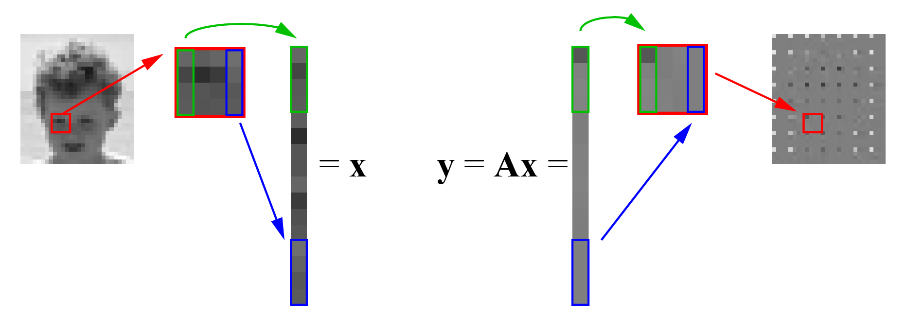
Linear mappings are common in real world engineering problems. One example is in image or video compression. Here an image to be coded is broken down to blocks, such as the $4 \times 4$ pixel blocks as shown in Figure 9.1.
Instead of encoding the brightness of each pixel in the block directly, a linear transform is applied to each block. The first step is to make a vector out of the $4\times 4$ block, by stacking every column of the block until a 16-dimensional vector $\vc{x}$ is obtained. This vector is now multiplied by a transformation matrix $\mx{A}$, which gives a new 16-dimensional vector $\vc{y} =\mx{A}\vc{x}$. This can now be unstacked to form a $4 \times 4$ image block. As can be seen in the figure, these transformed blocks are now much more similar to each other. The first value of the block changes a lot, but most of the others are close to zero (gray in the image). This means that they can either be ignored (set to zero) or be represented cheaply in terms of bits. The decoder obtains $\hat{\vc{y}}$, which is an approximate version of $\vc{y}$ since some values may have been set to zero or otherwise been approximated. The decoder then performs the opposite transformation $\hat{\vc{x}} =\mx{A}^{-1} \hat{\vc{y}}$ recover an approximate version of the pixel brightness values.
A real encoder is more complicated than this picture, and contain many optimizations. For instance, the linear mapping is not implemented using a matrix multiplication, but in a faster way that is mathematically equivalent to it.
 In Interactive Illustration 9.2, we show an example of how the variability changes
as over an image.
In Interactive Illustration 9.2, we show an example of how the variability changes
as over an image.
Linear mappings are common in real world engineering problems. One example is in image or video compression. Here an image to be coded is broken down to blocks, such as the $4 \times 4$ pixel blocks as shown in Figure 9.1.
Instead of encoding the brightness of each pixel in the block directly, a linear transform is applied to each block. The first step is to make a vector out of the $4\times 4$ block, by stacking every column of the block until a 16-dimensional vector $\vc{x}$ is obtained. This vector is now multiplied by a transformation matrix $\mx{A}$, which gives a new 16-dimensional vector $\vc{y} =\mx{A}\vc{x}$. This can now be unstacked to form a $4 \times 4$ image block. As can be seen in the figure, these transformed blocks are now much more similar to each other. The first value of the block changes a lot, but most of the others are close to zero (gray in the image). This means that they can either be ignored (set to zero) or be represented cheaply in terms of bits. The decoder obtains $\hat{\vc{y}}$, which is an approximate version of $\vc{y}$ since some values may have been set to zero or otherwise been approximated. The decoder then performs the opposite transformation $\hat{\vc{x}} =\mx{A}^{-1} \hat{\vc{y}}$ recover an approximate version of the pixel brightness values.
A real encoder is more complicated than this picture, and contain many optimizations. For instance, the linear mapping is not implemented using a matrix multiplication, but in a faster way that is mathematically equivalent to it.
Figure 9.1:
Simplified schematic of an image coder. The image is divided into blocks, and each block is transformed using a linear mapping. After the transformation the blocks contain many values close to zero (gray in the image) and thus become easy to compress.
Interactive Illustration 9.2:
Left: original image. Middle: $4 \times 4$ pixel area to be transformed. Right: after transform. Drag the mouse over the image (or touch it on a mobile device) to change the $4\times 4$ area that is transformed. Notice how much less the transformed area changes compared to the pixels. This reduced variability translates into reduced bits after compression.
Interactive Illustration 9.2:
Left: original image. Middle: $\hid{4 \times 4}$ pixel area to be transformed. Right: after transform. Drag the mouse over the image (or touch it on a mobile device) to change the $\hid{4\times 4}$ area that is transformed. Notice how much less the transformed area changes compared to the pixels. This reduced variability translates into reduced bits after compression.
We will start out this chapter by rehearsing what a mapping or a function for regular real values (scalars), and then move to vector mappings.
Definition 9.1:
Mapping
A mapping $F$ is a rule that, for every item in one set $N$, provides one item in another set $M$
This may look abstract, but in fact you have already been dealing with
mappings, but under the name functions. Another way to state
the same thing is
A mapping $F$ is a rule that, for every item in one set $N$, provides one item in another set $M$
| \begin{equation} F: N \rightarrow M. \end{equation} | (9.1) |
| \begin{equation} y = F(x). \end{equation} | (9.2) |
| \begin{equation} F: x \rightarrow y, x \in N. \end{equation} | (9.3) |
$y = x^2$
Interactive Illustration 9.3:
The function $\hid{y=x^2}$ is an example of a mapping from the real numbers $\hid{N = \mathbb{R}}$ to the set of real numbers $\hid{M = \mathbb{R}}$.
Interactive Illustration 9.4:
The curve above cannot be the graph of a function $\hid{y=f(x)}$ since there are two $\hid{y}$-values for some $\hid{x}$-values, such as $\hid{x=1}$.
Definition 9.2:
Domain, Codomain, and Range of a Mapping
Assume we have a mapping $y = F(x)$ where $x \in N$ and $y \in M$. Then $N$ is the domain of the mapping, and $M$ is the codomain of the mapping. The range (or alternatively, the image) of the mapping is the set $V_F$, where
The vertical bar should be read as "such that" or "with the property of". In this example, the expression can be read out as
"$V_F$ is the set of all elements $F(x)$ such that $x$ belongs to the set $N$".
For the example $y=x^2$, the range equals the set of positive real
numbers including zero, $V_F = \mathbb{R}_{\geq 0}$. Therefore, in this case, we only reach a subset of the codomain, i.e., $V_F$ is a subset of $M$.
Assume we have a mapping $y = F(x)$ where $x \in N$ and $y \in M$. Then $N$ is the domain of the mapping, and $M$ is the codomain of the mapping. The range (or alternatively, the image) of the mapping is the set $V_F$, where
| \begin{equation} V_F = \{F(x) | x \in N\}. \end{equation} | (9.4) |
In linear algebra, the inputs and outputs of a function are vectors instead of scalar. Assume we have a coordinate system $\vc{e}_1,\vc{e}_2$ and that $\begin{pmatrix}x_1 \\ x_2 \\\end{pmatrix}$ is the coordinate for the vector $\vc{x}$. We can now have a function $\vc{y} = F( \vc{x} )$ that maps every $\vc{x}$ to a new vector $\vc{y} = \begin{pmatrix}y_1 \\ y_2 \\\end{pmatrix}$ according to, for instance,
| \begin{equation} \begin{cases} y_1 = x_1 \\ y_2 = 0 \end{cases} \end{equation} | (9.5) |
$\vc{x}$
$\vc{y}$
$\vc{e}_1$
$\vc{e}_2$
Interactive Illustration 9.5:
The range, or image, of the function $\hid{F}$ in this case is the x-axis (marked with green), since all outputs of the function land on the $\hid{x}$-axis.
A slightly more interesting example of a mapping is the following
| \begin{equation} \begin{cases} y_1 = \cos(\frac{\pi}{3}) x_1 - \sin(\frac{\pi}{3}) x_2, \\ y_2 = \sin(\frac{\pi}{3}) x_1 + \cos(\frac{\pi}{3}) x_2. \end{cases} \end{equation} | (9.6) |
$\vc{x}$
$\vc{y}$
$\vc{e}_1$
$\vc{e}_2$
Interactive Illustration 9.6:
An example of a mapping from $\hid{\vc{x}}$ (red vector) to $\hid{\vc{y}}$ (blue vector). As can be seen, the vector is rotated $\hid{\frac{\pi}{3}}$ around the origin.
As can be seen by playing around with Interactive Ilustration 9.6, the output vector is a rotated copy of the input vector with the rotation angle $\frac{\pi}{3}$. As a matter of fact, we can write Equation (9.6) in matrix form as
| \begin{equation} \begin{pmatrix} y_1 \\ y_2 \end{pmatrix} = \left(\begin{array}{rr} \cos \frac{\pi}{3} & -\sin \frac{\pi}{3} \\ \sin \frac{\pi}{3} & \cos \frac{\pi}{3} \end{array}\right) \begin{pmatrix} x_1 \\ x_2 \end{pmatrix} \end{equation} | (9.7) |
| \begin{equation} \vc{y} = \mx{A} \vc{x}. \end{equation} | (9.8) |
The example in Interactive Illustration 9.3 can also be written in matrix form,
| \begin{equation} \begin{pmatrix} y_1 \\ y_2 \end{pmatrix} = \left(\begin{array}{rr} 1 & 0 \\ 0 & 0 \end{array}\right) \begin{pmatrix} x_1 \\ x_2 \end{pmatrix}, \end{equation} | (9.9) |
| \begin{equation} \begin{cases} y_1 = x_1 x_2 + x_2\\ y_2 = x_1 + e^{x_2} \end{cases} \end{equation} | (9.10) |
Definition 9.3:
Linear Mapping
A linear mapping is a mapping $F$, which satisfies
The intuitive description of the first condition is that it shouldn't
matter if you take the function of the sum or the sum of the
functions, you get the same result. The second condition states that
amplifying the input by a certain amount gives the same result as
amplifying the output by the same amount.
A linear mapping is a mapping $F$, which satisfies
| \begin{equation} \begin{cases} F( \vc{x}' + \vc{x}'') = F(\vc{x}') + F(\vc{x}''), \\ F( \lambda \vc{x} ) = \lambda F(\vc{x}). \\ \end{cases} \end{equation} | (9.11) |
Example 9.2:
Shopping Cart to Cost
Assume that a shop only sells packages of penne, jars of Arrabiata sauce, and bars of chocolate. The contents of your shopping cart can be modelled as a vector space. Introduce addition of two shopping carts as putting all of the items of both carts in one cart. Introduce multiplication of a scalar as multiplying the number of items in a shopping cart with that scalar. Notice that here, there are practical problems with multiplying a shopping cart with non-integer numbers or negative numbers, which makes the model less useful in practice. Introduce a set of basis shopping carts. Let $\vc{e}_1$ correspond to the shopping cart containing one package of penne, let $\vc{e}_2$ correspond to the shopping cart containing one jar of Arrabiata sauce, and let $\vc{e}_3$ correspond to the shopping cart containing one bar of chocolate. Then each shopping cart $\vc{x}$ can be described by three coordinates $(x_1, x_2, x_3)$ such that $\vc{x} = x_1 \vc{e}_1 + x_2 \vc{e}_2 + x_3 \vc{e}_3$.
There is a mapping from shopping carts $\vc{x}$ to price $y \in \R$. We can introduce the matrix $\vc{A} = \begin{pmatrix}a_{11} & a_{12} & a_{13} \end{pmatrix}$ where $a_{11}$ is the price of a package of penne, $a_{12}$ is the price of a jar of Arrabiata sauce and $a_{13}$ is the price of a bar of chocolate. The price $y$ can now be expressed as $y = \mx{A} \vc{x}$.
In real life this map is often non-linear, e.g., a shop might have campaigns saying 'buy 3 for the price of 2'. But modelling the mapping as a linear map is often a reasonable and useful model. Again (as is common with mathematical modelling) there is a discrepancy between mathematical model and reality. The results of mathematical analysis must always be used with reason and critical thinking. Even if the cost of a shopping cart of 1 package of penne is 10, it does not always mean that you can sell packages of penne to the store for 10 each.
Theorem 9.1:
Matrix Form of Linear Mappings
A mapping $\vc{y} = F(\vc{x})$ can be written in the form $\vc{y} = \mx{A}\vc{x}$ (matrix form) if and only if it is linear.
A mapping $\vc{y} = F(\vc{x})$ can be written in the form $\vc{y} = \mx{A}\vc{x}$ (matrix form) if and only if it is linear.
To prove the theorem we need to prove both directions, that every linear mapping can be written as $\vc{y} = \mx{A}\vc{x}$, and that every mapping $\vc{y} = \mx{A}\vc{x}$ is linear. We will do this for the case when both $\vc{x}$ and $\vc{y}$ are two-dimensional mappings, but a similar proof works for any dimensionality of both $\vc{x}$ and $\vc{y}$.
Assume we have a basis $\vc{e}_1$,$\vc{e}_2$ in $N$ and $M$. We can then write the input $\vc{x}$ and the output $\vc{y}$ in this basis,
| \begin{align} \vc{x} & = x_1 \vc{e}_1 + x_2 \vc{e}_2,\\ \vc{y} & = y_1 \vc{e}_1 + y_2 \vc{e}_2.\\ \end{align} | (9.12) |
| \begin{equation} \vc{y} = F(\vc{x}) = F(x_1 \vc{e}_1 + x_2 \vc{e}_2), \end{equation} | (9.13) |
| \begin{equation} \vc{y} = F(x_1 \vc{e}_1) + F(x_2 \vc{e}_2) = x_1F(\vc{e}_1) + x_2F(\vc{e}_2). \end{equation} | (9.14) |
| \begin{equation} F(\vc{e}_1) = a_{11}\vc{e}_1 + a_{21}\vc{e}_2. \end{equation} | (9.15) |
| \begin{equation} F(\vc{e}_2) = a_{12}\vc{e}_1 + a_{22}\vc{e}_2. \end{equation} | (9.16) |
| \begin{equation} \vc{y} = x_1(a_{11}\vc{e}_1 + a_{21}\vc{e}_2) + x_2(a_{12}\vc{e}_1 + a_{22}\vc{e}_2) = \\ (x_1 a_{11} + x_2 a_{12})\vc{e}_1 + (x_1 a_{21} + x_2 a_{22})\vc{e}_2 \\ \end{equation} | (9.17) |
| \begin{equation} \begin{pmatrix} y_1 \\ y_2 \end{pmatrix} = \left(\begin{array}{rr} a_{11} & a_{12} \\ a_{21} & a_{22} \end{array}\right) \begin{pmatrix} x_1 \\ x_2 \end{pmatrix} \end{equation} | (9.18) |
| \begin{equation} \vc{y} = \mx{A}\vc{x}. \end{equation} | (9.19) |
| \begin{equation} F(\vc{x}' + \vc{x}'') = \mx{A}(\vc{x}' + \vc{x}'') = \mx{A}\vc{x}' + \mx{A}\vc{x}'' = F(\vc{x}') + F(\vc{x}''). \end{equation} | (9.20) |
| \begin{equation} F(\lambda \vc{x'}) = \mx{A}(\lambda \vc{x}') = \lambda \mx{A} \vc{x}' = \lambda F(\vc{x'}) \end{equation} | (9.21) |
$\square$
It is often the case that you want to find the matrix $\mx{A}$ for a particular linear mapping. Then the following theorem can be of great help.
Theorem 9.2:
Mapping of Basis Vectors
For a linear mapping $\vc{y} = F(\vc{x})$ written on the form $\vc{y} = \mx{A}\vc{x}$ in the base $\vc{e}_1, \ \vc{e}_2, \ \ldots, \ \vc{e}_n$, the column vectors of $\mx{A}$ are the images of the basis vectors, $\vc{a}_{,1} = F(\vc{e}_1), \ \vc{a}_{,2} = F(\vc{e}_2), \ \ldots, \ \vc{a}_{,n} = F(\vc{e}_n)$.
For a linear mapping $\vc{y} = F(\vc{x})$ written on the form $\vc{y} = \mx{A}\vc{x}$ in the base $\vc{e}_1, \ \vc{e}_2, \ \ldots, \ \vc{e}_n$, the column vectors of $\mx{A}$ are the images of the basis vectors, $\vc{a}_{,1} = F(\vc{e}_1), \ \vc{a}_{,2} = F(\vc{e}_2), \ \ldots, \ \vc{a}_{,n} = F(\vc{e}_n)$.
We will prove the case when $N = M = 3$, but the proof for other values of $M$ and $N$ is similar.
The first basis vector $\vc{e}_1$ can be written as $\vc{e}_1 = 1 \vc{e}_1 + 0\vc{e}_2 + 0 \vc{e}_3$ and thus has the coordinates $(1, 0, 0)$. Using $\vc{x} = \begin{pmatrix} 1 \\ 0 \\ 0\end{pmatrix}$ in the formula $\vc{y} = \mx{A}\vc{x}$ gives
| \begin{equation} \begin{pmatrix} y_1 \\ y_2 \\ y_3\end{pmatrix} = \left(\begin{array}{rrr} a_{11} & a_{12} & a_{13}\\ a_{21} & a_{22} & a_{23}\\ a_{31} & a_{32} & a_{33}\\ \end{array}\right) \begin{pmatrix} 1 \\ 0 \\ 0 \end{pmatrix} = \left(\begin{array}{r} 1 a_{11} + 0 a_{12} + 0 a_{13}\\ 1 a_{21} + 0 a_{22} + 0 a_{23}\\ 1 a_{31} + 0 a_{32} + 0 a_{33}\\ \end{array}\right) = \begin{pmatrix} a_{11} \\ a_{21} \\ a_{31} \end{pmatrix}, \end{equation} | (9.22) |
| \begin{equation} \left(\begin{array}{rrr} a_{11} & a_{12} & a_{13}\\ a_{21} & a_{22} & a_{23}\\ a_{31} & a_{32} & a_{33}\\ \end{array}\right) \begin{pmatrix} 0 \\ 1 \\ 0 \end{pmatrix} = \left(\begin{array}{r} 0 a_{11} + 1 a_{12} + 0 a_{13}\\ 0 a_{21} + 1 a_{22} + 0 a_{23}\\ 0 a_{31} + 1 a_{32} + 0 a_{33}\\ \end{array}\right) = \begin{pmatrix} a_{12} \\ a_{22} \\ a_{32} \end{pmatrix}, \end{equation} | (9.23) |
| \begin{equation} \left(\begin{array}{rrr} a_{11} & a_{12} & a_{13}\\ a_{21} & a_{22} & a_{23}\\ a_{31} & a_{32} & a_{33}\\ \end{array}\right) \begin{pmatrix} 0 \\ 0 \\ 1 \end{pmatrix} = \left(\begin{array}{r} 0 a_{11} + 0 a_{12} + 1 a_{13}\\ 0 a_{21} + 0 a_{22} + 1 a_{23}\\ 0 a_{31} + 0 a_{32} + 1 a_{33}\\ \end{array}\right) = \begin{pmatrix} a_{13} \\ a_{23} \\ a_{33} \end{pmatrix}, \end{equation} | (9.24) |
$\square$
We can now use this fact to easily find the matrix $\mx{A}$ for a linear mapping by simply observing what happens to the basis function.
Example 9.3:
Finding a Linear Mapping's Matrix
A linear mapping $\vc{y} = F(\vc{x})$ rotates a two-dimensional vector $\vc{x}$ counterclockwise 90 degrees. Find the transformation matrix $\mx{A}$ of the matrix form $\vc{y} = \mx{A} \vc{x}$ when the standard orthonormal basis $\vc{e}_1=(1,0)$, $\vc{e}_2=(0,1)$ is used.
The first column vector of $\mx{A}$ will be the image of the first basis vector $\vc{e}_1$, which is the $x$-axis. Rotating that 90 degrees counterclockwise brings it parallel with the $y$-axis, which has coordinates $(0, 1)$. Thus the first column vector is $\vc{a}_{,1}= \begin{pmatrix} 0 \\ 1 \end{pmatrix}$.
The second column vector will be the image of the second basis vector, which is the $y$-axis. Rotating the $y$-axis 90 degrees counter clockwise makes it ending up in $(-1, 0)$. The second column vector is thus $\vc{a}_{,1} = \begin{pmatrix} -1 \\ 0 \end{pmatrix}$ and we can write $\mx{A}$ as
This is shown in Interactive Illustration 9.7.
A linear mapping $\vc{y} = F(\vc{x})$ rotates a two-dimensional vector $\vc{x}$ counterclockwise 90 degrees. Find the transformation matrix $\mx{A}$ of the matrix form $\vc{y} = \mx{A} \vc{x}$ when the standard orthonormal basis $\vc{e}_1=(1,0)$, $\vc{e}_2=(0,1)$ is used.
The first column vector of $\mx{A}$ will be the image of the first basis vector $\vc{e}_1$, which is the $x$-axis. Rotating that 90 degrees counterclockwise brings it parallel with the $y$-axis, which has coordinates $(0, 1)$. Thus the first column vector is $\vc{a}_{,1}= \begin{pmatrix} 0 \\ 1 \end{pmatrix}$.
The second column vector will be the image of the second basis vector, which is the $y$-axis. Rotating the $y$-axis 90 degrees counter clockwise makes it ending up in $(-1, 0)$. The second column vector is thus $\vc{a}_{,1} = \begin{pmatrix} -1 \\ 0 \end{pmatrix}$ and we can write $\mx{A}$ as
| \begin{equation} \mx{A} = \left(\begin{array}{rr} 0 & -1 \\ 1 & 0 \\ \end{array}\right) . \end{equation} | (9.25) |
$\textcolor{#aa0000}{\vc{e}_1 = \left(\begin{array}{c} 1 \\ 0\\ \end{array}\right)}$
$\textcolor{#0000aa}{\vc{F}(\vc{e}_1) = \left(\begin{array}{c} 0 \\ 1\\ \end{array}\right)}$
$\begin{array}{rr} \textcolor{#0000aa}{0} & \hid{-1} \\ \textcolor{#0000aa}{1} & \hid{0} \\ \end{array}$
$\begin{array}{rr} \textcolor{#0000aa}{0} & \hid{-1} \\ \textcolor{#0000aa}{1} & \hid{0} \\ \end{array}$
$\begin{array}{rr} \hid{0} & \textcolor{#00aa00}{-1} \\ \hid{1} & \textcolor{#00aa00}{0} \\ \end{array}$
$\textcolor{#aa0000}{\vc{e}_2 = \left(\begin{array}{c} 0 \\ 1\\ \end{array}\right)}$
$\textcolor{#00aa00}{\vc{F}(\vc{e}_2) = \left(\begin{array}{r} -1 \\ 0\\ \end{array}\right)}$
$\vc{y} = \left(\begin{array}{rr} \hid{0} & \hid{-1} \\ \hid{1} & \hid{0} \\ \end{array}\right) \vc{x}$
Interactive Illustration 9.7:
To get the transformation matrix $\hid{\mx{A}}$ of a $\hid{90}$-degree counterclockwise rotation, we start with the first basis vector $\hid{\vc{e}_1 = \left(\begin{array}{c}1\\0\\ \end{array}\right)}$ marked in red.
Assume we have a linear mapping $\vc{y} = F(\vc{x})$, and that the output vector $\vc{y}$ can be fed into another linear mapping $\vc{z}= G(\vc{y})$. For this to work we need the domain of $G$ to be equal the codomain of $F$. As an example, if $G(\vc{y})$ accepts two-dimensional vectors, i.e., the domain of $G$ is $\mathbb{R}^2$, then the output of $F$, must be a two-dimensional vector, i.e., the codomain of $F(\vc{x})$ must also be $\mathbb{R}^2$. We then call the mapping
| \begin{equation} \vc{z} = G(F(\vc{x})) \end{equation} | (9.26) |
Theorem 9.3:
Composition of Linear Mappings
If $\vc{y} = F(\vc{x})$ and $\vc{z} = G(\vc{y})$ are both linear mappings then the composite mapping $\vc{z} = G(F(\vc{x}))$ is also linear.
If $\vc{y} = F(\vc{x})$ and $\vc{z} = G(\vc{y})$ are both linear mappings then the composite mapping $\vc{z} = G(F(\vc{x}))$ is also linear.
Since $\vc{y} = F(\vc{x})$ is a linear mapping, it can be written on matrix from $\vc{y} = \mx{A}\vc{x}$, and likewise can $\vc{z} = G(\vc{y})$ be written as $\vc{z} = \mx{B}\vc{y}$. We can then write
| \begin{equation} \vc{z} = \mx{B}\vc{y} = \mx{B}(\mx{A}\vc{x}) = (\mx{B}\mx{A})\vc{x} = \mx{C}\vc{x}, \end{equation} | (9.27) |
$\square$
Example 9.4:
Composition of Linear Mappings
Find a mapping $F$ that rotates a two-dimensional vector by 30 degrees, and then multiplies the $x$-coordinate by two.
We split this into two parts. First we find a mapping $\vc{y} =G(\vc{x})$ that rotates 30 degrees, and then another mapping $\vc{z} = H(\vc{y})$ that doubles the $x$-coordinate.
Let $\mx{A}$ be the transformation matrix for $G$. We know from Definition 6.10 that a rotation by $\phi$ is obtained by $ \left(\begin{array}{rr} \cos \phi & -\sin \phi \\ \sin \phi & \cos \phi \end{array}\right).$ Thus, setting $\phi = \frac{\pi}{6}$, we get
Let $\mx{B}$ be the transformation matrix for $H$. The task of this is
to double the $x$-coordinate, but leave the $y$-coordinate intact. This can be solved by setting
Finally, the transformation matrix $\mx{C}$ for the composite mapping $\vc{z} = H(G(\mx{x}))$ is
Find a mapping $F$ that rotates a two-dimensional vector by 30 degrees, and then multiplies the $x$-coordinate by two.
We split this into two parts. First we find a mapping $\vc{y} =G(\vc{x})$ that rotates 30 degrees, and then another mapping $\vc{z} = H(\vc{y})$ that doubles the $x$-coordinate.
Let $\mx{A}$ be the transformation matrix for $G$. We know from Definition 6.10 that a rotation by $\phi$ is obtained by $ \left(\begin{array}{rr} \cos \phi & -\sin \phi \\ \sin \phi & \cos \phi \end{array}\right).$ Thus, setting $\phi = \frac{\pi}{6}$, we get
| \begin{equation} \mx{A} = \left(\begin{array}{rr} \frac{\sqrt{3}}{2} & -\frac{1}{2} \\ \frac{1}{2} & \frac{\sqrt{3}}{2} \end{array}\right). \end{equation} | (9.28) |
| \begin{equation} \mx{B} = \left(\begin{array}{rr} 2 & 0 \\ 0 & 1 \end{array}\right). \end{equation} | (9.29) |
| \begin{equation} \mx{C} = \mx{B}\mx{A} =\left(\begin{array}{rr} 2 & 0 \\ 0 & 1 \end{array}\right) \left(\begin{array}{rr} \frac{\sqrt{3}}{2} & -\frac{1}{2} \\ \frac{1}{2} & \frac{\sqrt{3}}{2} \end{array}\right) = \left(\begin{array}{rr} \sqrt{3} & -1 \\ \frac{1}{2} & \frac{\sqrt{3}}{2} \end{array}\right). \end{equation} | (9.30) |
For some mappings, several inputs $\vc{x}$ can map to the same value $F(\vc{x})$. As an example, in Interactive Illustration 9.5, where we simply project a point onto the $x$-axis by setting the $y$-coordinate to zero, both $\vc{x}_1 = (1,5)$ and $\vc{x}_2 = (1,2)$ will map to the same point $(1,0) = F(\vc{x}_1) =F(\vc{x}_2)$. However, for some mappings, the result will be unique, so if we start out with two different $\vc{x}_1 \neq \vc{x}_2$, we know that $F(\vc{x}_1) \neq F(\vc{x}_2)$. We call such mappings injective.
Definition 9.4:
Injective mappings
A mapping $y = F(x)$ is injective, if any two different vectors $\vc{x}_1 \neq \vc{x}_2$ will always give rise to two different images $F(\vc{x}_1) \neq F(\vc{x}_2)$.
Another way to state this is to say that an injective mapping has the property that if two images $F(\vc{x}_1)$ and $F(\vc{x}_2)$ are equal, then $\vc{x_1}$ must equal $\vc{x_2}$.
A mapping $y = F(x)$ is injective, if any two different vectors $\vc{x}_1 \neq \vc{x}_2$ will always give rise to two different images $F(\vc{x}_1) \neq F(\vc{x}_2)$.
For some mappings $\vc{y} = F(\vc{x})$, we can reach every point $\vc{y}$ in the codomain by selecting a suitable $\vc{x}$. When the range of the mapping covers the codomain like this, we call the mapping surjective. A mapping that is both injective and surjective is called bijective.
Definition 9.5:
Surjective mapping
A mapping $\vc{y} =F(\vc{x})$, where $\vc{x} \in N$ and $\vc{y} \in M$ is surjective if the range $V_F$ is equal to to the codomain $M$, $V_F = M$.
A mapping $\vc{y} =F(\vc{x})$, where $\vc{x} \in N$ and $\vc{y} \in M$ is surjective if the range $V_F$ is equal to to the codomain $M$, $V_F = M$.
Definition 9.6:
Bijective mapping
A mapping is bijective if it is both injective and surjective.
We will now go through a few examples of mappings and investigate whether they are injective, surjective, and bijective.
A mapping is bijective if it is both injective and surjective.
Example 9.5:
Type of Mapping I
Consider the mapping $\vc{y} = F(\vc{x})$
where $\vc{x}$ belongs to the domain $N = \mathbb{R}^2$ and the
resulting vector $\vc{y}$ belongs to the codomain $M =\mathbb{R}^2$. This mapping is injective, since if we have two
different input values $\vc{a}$ and $\vc{b}$, the output vector
$\begin{pmatrix}e^{a_1}\\e^{a_2}\end{pmatrix}$ will be different from
$\begin{pmatrix}e^{b_1}\\e^{b_2}\end{pmatrix}$ unless $\vc{a} =\vc{b}$. However, the mapping is not surjective, since it is
impossible to reach negative values for $y_1$ and $y_2$ ($e^x > 0$ for
all real values of $x$). The range $V_F$ is in this case only the
quadrant $y_1 > 0, y_2 > 0$ and not equal to the codomain $M =\mathbb{R}^2$. Since the mapping is not surjective, it is also not
bijective.
Consider the mapping $\vc{y} = F(\vc{x})$
| \begin{equation} \begin{pmatrix} y_1 \\ y_2 \end{pmatrix} = F\left(\begin{pmatrix} x_1 \\ x_2 \end{pmatrix}\right) = \left(\begin{array}{r} e^{x_1} \\ e^{x_2} \end{array}\right) , \end{equation} | (9.31) |
Example 9.6:
Type of Mapping II
Investigate whether the mapping $\vc{y} = F(\vc{x})$
is bijective. In this case both the domain $N$ and the codomain $M$ equals the plane of real numbers $\mathbb{R}^2$.
First we investigate whether it is injective. It is clear that it is, since two different input values $\vc{a}$ and $\vc{b}$ will generate two different output vectors $\begin{pmatrix}2 a_1\\3a_2\end{pmatrix} \neq \begin{pmatrix}2b_1\\3b_2\end{pmatrix}$ unless $\vc{a} = \vc{b}$.
Also all output vectors $\begin{pmatrix}y_1\\y_2\end{pmatrix}$ (the entire codomain $M = \mathbb{R}^2$) can be reached by using the input $\begin{pmatrix}x_1\\ x_2\end{pmatrix}= \begin{pmatrix}\frac{y_1}{2}\\\frac{y_2}{3}\end{pmatrix}$. This means that the mapping is also surjective. Since the mapping is both injective and surjective, it is bijective.
As it turns out, linear mappings that are bijective have many useful properties. As an example, it is simple to find the inverse mapping, as we will see in the following theorem.
Investigate whether the mapping $\vc{y} = F(\vc{x})$
| \begin{equation} \begin{pmatrix} y_1 \\ y_2 \end{pmatrix} = F\left(\begin{pmatrix} x_1 \\ x_2 \end{pmatrix}\right) = \left(\begin{array}{r} 2 x_1 \\ 3 x_2 \end{array}\right) \end{equation} | (9.32) |
First we investigate whether it is injective. It is clear that it is, since two different input values $\vc{a}$ and $\vc{b}$ will generate two different output vectors $\begin{pmatrix}2 a_1\\3a_2\end{pmatrix} \neq \begin{pmatrix}2b_1\\3b_2\end{pmatrix}$ unless $\vc{a} = \vc{b}$.
Also all output vectors $\begin{pmatrix}y_1\\y_2\end{pmatrix}$ (the entire codomain $M = \mathbb{R}^2$) can be reached by using the input $\begin{pmatrix}x_1\\ x_2\end{pmatrix}= \begin{pmatrix}\frac{y_1}{2}\\\frac{y_2}{3}\end{pmatrix}$. This means that the mapping is also surjective. Since the mapping is both injective and surjective, it is bijective.
Theorem 9.4:
Equivalence of Inverse Mapping
For a linear mapping $\vc{y} = F(\vc{x})$ from $\vc{x} \in \mathbb{R}^n$ to $\vc{y} \in \mathbb{R}^n$, the following three statements are equivalent:
For a linear mapping $\vc{y} = F(\vc{x})$ from $\vc{x} \in \mathbb{R}^n$ to $\vc{y} \in \mathbb{R}^n$, the following three statements are equivalent:
- The mapping $F$ is bijective.
- The transformation matrix for $F$ is invertible.
- The images $F(\vc{e}_1), \ldots, F(\vc{e}_n)$ of the basis vectors $\vc{e}_1, \, \ldots, \, \vc{e}_n$ constitute a basis in $\mathbb{R}^n$.
i $\rightarrow$ ii: If the mapping $F$ is bijective, this means that the equation $F(\vc{x}) = \vc{y}$ has a unique solution $\vc{x}$ for every $\vc{y}$. Specifically, since $F$ is injective, we know that if $F(\vc{u})=F(\vc{v})$, $\vc{u}$ must be equal to $\vc{v}$. Also, since $F$ is surjective, every $\vc{y}$ can be reached with the proper $\vc{x}$. The matrix form of $F$ is $\vc{y} = \mx{A}\vc{x}$, and that this equation has a unique solution for every $\vc{y}$ is equivalent to saying that $\mx{A}$ is invertible according to Theorem 6.9.
ii $\rightarrow$ iii: According to Theorem 9.2, $F(\vc{e}_1)$ is just the first column of $\mx{A}$. Likewise, $F(\vc{e}_2)$ is the second column of $\mx{A}$, and so on. Theorem 6.9 tells us that if $\mx{A}$ is invertible, the columns of $\mx{A}$ span $\mathbb{R}^n$, which means that they form a basis in $\mathbb{R}^n$.
iii $\rightarrow$ i: We first prove that iii means that $F$ is injective, i.e., that if $F(\vc{u}) = F(\vc{v})$ then $\vc{u}$ must equal $\vc{v}$.
We can write $\vc{u} = u_1 \vc{e}_1 + u_2 \vc{e}_2 + \ldots + u_n\vc{e}_n$ and $\vc{v} = v_1 \vc{e}_1 + v_2 \vc{e}_2 + \ldots + v_n\vc{e}_n$. We know that $F(\vc{u}) = F(\vc{v})$, hence $F(\vc{u})-F(\vc{v}) = \vc{0}$, which is equivalent to
| \begin{equation} F(u_1 \vc{e}_1 + u_2 \vc{e}_2 + \ldots + u_n\vc{e}_n) - F(v_1 \vc{e}_1 + v_2 \vc{e}_2 + \ldots + v_n\vc{e}_n) = \vc{0}. \end{equation} | (9.33) |
| \begin{equation} u_1 F(\vc{e}_1) + u_2 F(\vc{e}_2) + \ldots + u_nF(\vc{e}_n) - \Big( v_1 F(\vc{e}_1) + v_2 F(\vc{e}_2) + \ldots + v_nF(\vc{e}_n)\Big) = \vc{0}. \end{equation} | (9.34) |
| \begin{equation} (u_1-v_1) F(\vc{e}_1) + (u_2 - v_2) F(\vc{e}_2) + \ldots + (u_n - v_n) F(\vc{e}_n) = \vc{0}, \end{equation} | (9.35) |
We then prove that $\vc{y} = F(\vc{x})$ is surjective, i.e., we can reach every $\vc{y}$ with a proper choice of $\vc{x}$.
We can write $\vc{x} = x_1\vc{e}_1 + x_2\vc{e}_2 + \ldots + x_n\vc{e}_n$, and hence $\vc{y} = F(\vc{x})$ can be written
| \begin{equation} \vc{y} = F(\vc{x}) = F(x_1\vc{e}_1 + x_2\vc{e}_2 + \ldots + x_n\vc{e}_n). \end{equation} | (9.36) |
| \begin{equation} \vc{y} = x_1F(\vc{e}_1) + x_2F(\vc{e}_2) + \ldots x_n F(\vc{e}_n), \end{equation} | (9.37) |
$\square$
From this proof, the following theorem follows.
Theorem 9.5:
Inverse Mapping Matrix
For a bijective linear mapping $\vc{y} = F(\vc{x})$ with transformation matrix $\mx{A}$, the inverse mapping $\vc{x} =F^{-1}(\vc{y})$ is linear and has the transformation matrix $\inv{\mx{A}}$.
For a bijective linear mapping $\vc{y} = F(\vc{x})$ with transformation matrix $\mx{A}$, the inverse mapping $\vc{x} =F^{-1}(\vc{y})$ is linear and has the transformation matrix $\inv{\mx{A}}$.
We are seeking a mapping $\inv{F}$ with the property that $\inv{F}(F(\vc{x})) = \vc{x}$.
Consider $\vc{y} = F(\vc{x})$ on matrix from
| \begin{equation} \vc{y} = \mx{A}\vc{x}. \end{equation} | (9.38) |
| \begin{equation} \inv{\mx{A}}\vc{y} = \inv{\mx{A}}\mx{A}\vc{x} = \mx{I} \vc{x} = \vc{x}, \end{equation} | (9.39) |
| \begin{equation} \vc{x} = \inv{\mx{A}} \vc{y}. \end{equation} | (9.40) |
$\square$
In Interactive Illustration 9.8, we show how linear mappings can be used to generate a shadow effect.
Example 9.7:
Shadows
Assume we have a plane that goes through the origin with the normal vector $\vc{n} = (0, 1, 0)$. Furthermore, assume the sun is infinitely far away from the origin, positioned in the direction $\vc{r} = (0.5,1.0, 0.25)$. We have a lot of points above the plane, and would like to know their shadows on the plane. Assume also that we have been reassured that this particular type of shadow projection can be expressed as a linear mapping.
It would be possible to calculate the shadow point by point, but it would be more convenient if we could create a linear mapping $\vc{y} =\mx{A}\vc{x}$ so that we could directly get the projected point $\vc{y}$ by simply multiplying the point $\vc{x}$ by the matrix $\mx{A}$. This should be possible, given that the problem is linear.
In this case, we take advantage of Theorem 9.2, i.e., to obtain $\mx{A}$ we only need to know what happens to the three unit vectors. The first column vector of the transformation matrix $\mx{A}$ is simply the image of the first unit vector $\vc{e_1} = (1,0,0)$, and so forth. Hence, if we find out where on the plane the shadow of the point $(1,0,0)$ lands, we have the first column of $\mx{A}$.
We can write the plane on the form $ax+by+cz+d = 0$, and since we know the normal is $(0, 1, 0)$ this simplifies to $y+d=0$. Furthermore, since the origin $(0, 0, 0)$ is contained in the plane, the equation further simplifies to $y=0$. We can now take the line that goes through the point $(p_x, p_y, p_z)$ and follow it in the direction of the sun, $(r_x, r_y, r_z)$,
Inserting this line equation into the plane equation should give us the distance $\lambda$ that we need to travel from $P$ to get to the intersection. When we insert it into the plane equation $y = 0$ we get $p_y + 1.0 \lambda = 0$. For the first unit vector $\vc{e}_1=(1, 0, 0)$, we have $p_y = 0$, giving $0 + \lambda = 0$, which means that $\lambda = 0$. The intersection point is therefore at
$(1, 0, 0) + 0\vc{r} = (1, 0, 0)$. This is therefore the first column of $\mx{A}$. For the second unit vector $\vc{e}_2 = (0, 1, 0)$, we have $p_y = 1$, giving the equation $1+\lambda = 0$, or $\lambda = -1$. Therefore the second column of $\mx{A}$ is $(0, 1, 0) + (-1)(0.5, 1.0, 0.25) = (-0.5, 0, -0.25)$. The third unit vector $\vc{e}_3 = (0, 0, 1)$ gets $\lambda = 0$ and hence the last column of $\mx{A}$ is $(0, 0, 1) - 0\vc{r} = (0, 0, 1)$.
In summary, we have now created a linear mapping $\vc{y} = \mx{A}\vc{x}$ that takes a point $\vc{x}$ and maps it to its shadow $\vc{y}$. The matrix $\mx{A}$ equals
This is used in the figure below. Each point of the cube is just projected to the plane using $\vc{y} = \mx{A}\vc{x}$ with the matrix $\mx{A}$ from above. By drawing each face of the cube using the projected coordinates instead of the original coordinates, it is possible to draw the shadow of the cube.
Now that we have this shadow example, we can investigate whether the mapping is bijective.
Assume we have a plane that goes through the origin with the normal vector $\vc{n} = (0, 1, 0)$. Furthermore, assume the sun is infinitely far away from the origin, positioned in the direction $\vc{r} = (0.5,1.0, 0.25)$. We have a lot of points above the plane, and would like to know their shadows on the plane. Assume also that we have been reassured that this particular type of shadow projection can be expressed as a linear mapping.
It would be possible to calculate the shadow point by point, but it would be more convenient if we could create a linear mapping $\vc{y} =\mx{A}\vc{x}$ so that we could directly get the projected point $\vc{y}$ by simply multiplying the point $\vc{x}$ by the matrix $\mx{A}$. This should be possible, given that the problem is linear.
In this case, we take advantage of Theorem 9.2, i.e., to obtain $\mx{A}$ we only need to know what happens to the three unit vectors. The first column vector of the transformation matrix $\mx{A}$ is simply the image of the first unit vector $\vc{e_1} = (1,0,0)$, and so forth. Hence, if we find out where on the plane the shadow of the point $(1,0,0)$ lands, we have the first column of $\mx{A}$.
We can write the plane on the form $ax+by+cz+d = 0$, and since we know the normal is $(0, 1, 0)$ this simplifies to $y+d=0$. Furthermore, since the origin $(0, 0, 0)$ is contained in the plane, the equation further simplifies to $y=0$. We can now take the line that goes through the point $(p_x, p_y, p_z)$ and follow it in the direction of the sun, $(r_x, r_y, r_z)$,
| \begin{equation} \begin{pmatrix} x \\ y \\ z \end{pmatrix}= \begin{pmatrix} p_x \\ p_y \\ p_z \end{pmatrix}+ \lambda \begin{pmatrix} r_x \\ r_y \\ r_z \end{pmatrix} = \begin{pmatrix} p_x \\ p_y \\ p_z \end{pmatrix}+ \lambda \begin{pmatrix} 0.5 \\ 1.0 \\ 0.25 \end{pmatrix}. \end{equation} | (9.41) |
In summary, we have now created a linear mapping $\vc{y} = \mx{A}\vc{x}$ that takes a point $\vc{x}$ and maps it to its shadow $\vc{y}$. The matrix $\mx{A}$ equals
| \begin{equation} \mx{A} = \left(\begin{array}{ccc} 1 & -0.5 & 0\\ 0 & 0 & 0\\ 0 & -0.25 & 1\\ \end{array}\right). \end{equation} | (9.42) |
$O$
$\vc{n}$
$\vc{r}$
$P$
$P'$
$\vc{x}$
$\vc{y}=\mx{A}\vc{x}$
Interactive Illustration 9.8:
In this illustration, we will show how a linear mapping can be used to create shadow effects. We start by constructing a linear mapping that projects a point $\hid{P}$ to $\hid{P}$', which is the projection on to the plane along the vector $\hid{\vc{r}}$.
Example 9.8:
Bijectivity of Shadows
Examine whether the mapping in in Example 9.7 is bijective.
According to Theorem 9.4, a mapping $\vc{y} = \mx{A}\vc{x}$ bijective if and only if the transformation matrix $\mx{A}$ is invertible. We know from Theorem 7.10 from the chapter on determinants that a matrix is invertible only if the determinant is nonzero. However, the determinant
must be zero since the second row is zero (see Theorem 7.1$(iv)$ combined with $(vii)$). Hence the mapping cannot be bijective.
This makes sense. If you know a set of points and the direction of the sun, you can calculate their respective shadows. However, if you only have the shadows and the direction of the sun, you cannot recover the original positions since you only know the direction in which the point is located and not the distance to it. Hence the operation is not reversible, or in formal terms, bijective.
Examine whether the mapping in in Example 9.7 is bijective.
According to Theorem 9.4, a mapping $\vc{y} = \mx{A}\vc{x}$ bijective if and only if the transformation matrix $\mx{A}$ is invertible. We know from Theorem 7.10 from the chapter on determinants that a matrix is invertible only if the determinant is nonzero. However, the determinant
| \begin{equation} \det(\mx{A}) = \left|\begin{array}{ccc} 1 & -0.5 & 0\\ 0 & 0 & 0\\ 0 & -0.25 & 1\\ \end{array}\right| \end{equation} | (9.43) |
This makes sense. If you know a set of points and the direction of the sun, you can calculate their respective shadows. However, if you only have the shadows and the direction of the sun, you cannot recover the original positions since you only know the direction in which the point is located and not the distance to it. Hence the operation is not reversible, or in formal terms, bijective.
Example 9.9:
Image compression revisited
In Example 9.1 we saw that a mapping $\vc{y} = \mx{A}\vc{x}$ was used as part of the compression process. Is this mapping likely to be bijective?
The answer is yes. In order to be useful, we want the decoded image to look the same as the original, at least if we spend enough bits. If we had a mapping that was not bijective, information would be lost in the transform step $\vc{y} = \mx{A}\vc{x}$. No matter how well we would preserve $\vc{y}$, i.e., no matter how many bits we would spend to describe $\vc{y}$, it would never be possible to recover $\vc{x}$. If the mapping is bijective, on the other hand, it is simple to recover $\vc{x}$ using $\vc{x} = \inv{\mx{A}}\vc{y}$.