Chapter 8: Rank
This chapter is about a concept called the rank, which is a property of a matrix. In fact, it reveals several aspects of a matrix. Some of the examples here may be shown for square matrices but everything in this chapter works for rectangular matrices, say of size $m \times n$. We start with an example from the application of structure from sound.
Example 8.1:
Structure from Sound
There are many examples from applied mathematics, which involves the concept of rank. One such example is the so called structure from sound problem. In this example, sounds are recorded at a number of stationary, but unknown, microphone positions. Unknown sounds are emitted at unknown positions and at unknown times. It turns out that it is still possible to calculate (i) where the microphones are, (ii) how the sound source has moved, and (iii) when the sound sources were emitted, just using the measured sound signals from the microphones. Here rank plays an important role.
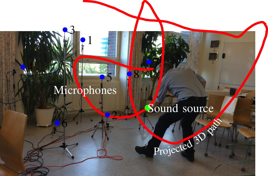 Figure 8.1 shows the measurement situation. Eight microphones capture the sound as a single sound source is moving in the room. The eight sound files are used to calculate the microphone positions and the sound source movement. See also the following YouTube clip.
The 3D sound source path and the microphone locations that are computed are also visualized in Interactive Illustration 8.2.
Figure 8.1 shows the measurement situation. Eight microphones capture the sound as a single sound source is moving in the room. The eight sound files are used to calculate the microphone positions and the sound source movement. See also the following YouTube clip.
The 3D sound source path and the microphone locations that are computed are also visualized in Interactive Illustration 8.2.
We start by explaining the null space, column space, and row space of a matrix. As will be shown these three spaces are themselves linear vector spaces. They are examples of linear subspaces, which are explained next.
There are many examples from applied mathematics, which involves the concept of rank. One such example is the so called structure from sound problem. In this example, sounds are recorded at a number of stationary, but unknown, microphone positions. Unknown sounds are emitted at unknown positions and at unknown times. It turns out that it is still possible to calculate (i) where the microphones are, (ii) how the sound source has moved, and (iii) when the sound sources were emitted, just using the measured sound signals from the microphones. Here rank plays an important role.
Figure 8.1:
Illustration of the measurement situation. The sound source (held in the left hand) is moving, while the eight microphones are stationary.
A linear subspace of a vector space is a subset of the vectors that is itself a linear space. To show that a subset of a linear space is a linear subspace one only has to check three things. This is captured by the following theorem.
Theorem 8.1:
Let $V$ be a linear vector space over the scalars $F$. (Here we will typically only use $F=\R $ or $F=\mathbb{C}$). A subset $W \subset V$ is a linear vector space, i.e. a subspace, if and only if $W$ satisfies the following three conditions:
Let $V$ be a linear vector space over the scalars $F$. (Here we will typically only use $F=\R $ or $F=\mathbb{C}$). A subset $W \subset V$ is a linear vector space, i.e. a subspace, if and only if $W$ satisfies the following three conditions:
- The zero vector $\vc{0} \in W$.
- If $\vc{v}_1 \in W$ and $\vc{v}_2 \in W$ then $\vc{v}_1+\vc{v}_2 \in W$.
- If $\vc{v} \in W$ and $\lambda \in F$ then $\lambda \vc{v}\in W$.
First, we prove that $W$ is a vector space if the conditions hold. By condition 1, we see that $W$ is nonempty. The conditions 2 and 3 ensure that the result of adding two vectors or multiplying a vector with a scalar does not take us outside the subset. Since the elements of $W$ are already part of vector space $V$, we then know that all the other rules of Theorem 2.1 hold.
Second, we prove that if the subset $W$ is a vector space then the three conditions must hold. Since $W$ is a vector space, then the properties 2 and 3 are satisfied. Since $W$ is non-empty, there is at least one element $\vc{w}$. We can then form $ \vc{0} = 0 \vc{w} \in W$. Thus property 1 holds.
$\square$
Example 8.2:
Let $\mx{A}$ be an $m \times n$ matrix. Let $V$ be the linear vector space $\R^n$. Let $W \subset V$ be the subset of vectors $\vc{v} \in V$ that fulfills $\mx{A}\vc{v} = \vc{0}$. Then $W$ is a linear vector space. This is true since
This means that the solutions to a homogeneous system is a linear space.
Let $\mx{A}$ be an $m \times n$ matrix. Let $V$ be the linear vector space $\R^n$. Let $W \subset V$ be the subset of vectors $\vc{v} \in V$ that fulfills $\mx{A}\vc{v} = \vc{0}$. Then $W$ is a linear vector space. This is true since
- The zero vector $\vc{0} \in W$ since $\mx{A}\vc{0} = \vc{0}$.
- If $\vc{v}_1 \in W$ and $\vc{v}_2 \in W$ then $\mx{A}(\vc{v}_1+\vc{v}_2) = \mx{A}\vc{v}_1+\mx{A}\vc{v}_2 = \vc{0}+\vc{0}$. Therefore $\vc{v}_1+\vc{v}_2 \in W$.
- If $\vc{v} \in W$ and $\lambda \in F$ then $\mx{A}(\lambda \vc{v}) = \lambda \mx{A} \vc{v}= \lambda\vc{0} =\vc{0}$. Therefore $\lambda \vc{v}\in W$.
Example 8.3:
Let $\mx{A}$ be an $m \times n$ matrix. Let $V$ be the linear vector space $\R^m$. Let $W \subset V$ be the subset of vectors $\vc{v} \in V$ that can be generated as $\vc{v}= \mx{A}\vc{u}$ for some $\vc{u} \in \R^n$. Then $W$ is a linear vector space. This is true since
This means that the set of linear combinations of a set of vectors is a linear space.
Let $\mx{A}$ be an $m \times n$ matrix. Let $V$ be the linear vector space $\R^m$. Let $W \subset V$ be the subset of vectors $\vc{v} \in V$ that can be generated as $\vc{v}= \mx{A}\vc{u}$ for some $\vc{u} \in \R^n$. Then $W$ is a linear vector space. This is true since
- The zero vector $\vc{0} \in W$ since $\vc{0}\in\R^m$ can be generated from $\vc{0} \in \R^n$ by $\vc{0} =\mx{A}\vc{0}$.
- If $\vc{v}_1 \in W$ and $\vc{v}_2 \in W$ then there exists $\vc{u}_1 \in \R^n$ and $\vc{u}_2 \in \R^n$ so that $\vc{v}_1 = \mx{A}\vc{u}_1$ and $\vc{v}_2 = \mx{A}\vc{u}_2$. But then $\vc{v}_1+\vc{v}_2 \in W$, since $(\vc{v}_1+\vc{v}_2) = \mx{A}\vc{u}_1+\mx{A}\vc{u}_2 = \mx{A}(\vc{u}_1 + \vc{u}_2)$.
- If $\vc{u} \in W$ and $\lambda \in F$ then there exists $\vc{u} \in \R^n$ so that $\vc{v} = \mx{A}\vc{u}$ . But then $\lambda \vc{v}\in W$ since $\lambda \vc{v} = \lambda \mx{A}(\vc{u}) = \mx{A} (\lambda \vc{u})$.
As we have seen in Section 5.5, a system of equations such as $\mx{A}\vc{x} = \vc{0}$ is called homogeneous. We will now show that the solutions to such systems reveal certain useful properties of $\mx{A}$. Let us start with an example. Assume we have a matrix
| \begin{equation} \mx{A} = \begin{pmatrix} 2 & \hid{-}5 & \hid{-}3 \\ 4 & \hid{-}2 & \hid{-}1 \\ 2 & -3 & -2 \end{pmatrix}, \end{equation} | (8.1) |
| \begin{equation} \begin{cases} \begin{array}{rrrl} 2 x_1 + 5 & \bs x_2 + 3 & \bs x_3 = 0, \\ 4 x_1 + 2 & \bs x_2 +\hid{3}& \bs x_3 = 0, \\ 2 x_1 - 3 & \bs x_2 - 2 & \bs x_3 = 0, \\ \end{array} \end{cases} \end{equation} | (8.2) |
| \begin{equation} \begin{cases} \begin{array}{rrrl} 2 x_1 + 5 & \bs x_2 + 3 & \bs x_3 = 0, \\ 8 & \bs x_2 + 5 & \bs x_3 = 0, \\ & & \bs 0 = 0. \\ \end{array} \end{cases} \end{equation} | (8.3) |
| \begin{equation} \vc{x}(t) = \begin{pmatrix} x_1 \\ x_2 \\ x_3 \end{pmatrix} = \begin{pmatrix} \frac{1}{16}t \\ -\frac{5}{8}t \\ t \end{pmatrix} \end{equation} | (8.4) |
Definition 8.1:
Null Space
If $\mx{A}$ is an $m\times n$ matrix (i.e., with $m$ rows and $n$ columns), then the entire set of solutions to $\mx{A}\vc{x}=\vc{0}$ is called the null space of $\mx{A}$.
By definition, the null space must be a subspace of $\R^n$, that is, $\nullity(\mx{A}) \leq n$.
It is a linear subspace, (see Example 8.2). The dimension of this subspace is important and has its own definition.
If $\mx{A}$ is an $m\times n$ matrix (i.e., with $m$ rows and $n$ columns), then the entire set of solutions to $\mx{A}\vc{x}=\vc{0}$ is called the null space of $\mx{A}$.
Definition 8.2:
Nullity
The dimension of the null space is denoted $\nullity(\mx{A})$.
Since the null space is a subspace of $\R^n$, we have $\nullity(\mx{A}) \leq n$. But how many dimensions lower is the null space? This is captured loosely by the number of constraints in $\mx{A}\vc{x}=\vc{0}$, however, here we must be careful. Just because there are $m$ equations in $\mx{A}\vc{x}=\vc{0}$ it does not automatically mean that $\nullity(\mx{A}) = n - m$. How many constraints there are in $\mx{A}$ is precisely what is captured by the concept of rank. What we are later going to show is that $\nullity(\mx{A}) = n - r$, i.e., that the dimension is lowered by $r$ (i.e., the rank of $\mx{A}$) using the constraints in $\mx{A}\vc{x}=\vc{0}$.
The dimension of the null space is denoted $\nullity(\mx{A})$.
Definition 8.3:
Null Vectors
Let $\vc{p}_1, \ldots, \vc{p}_k$ be a basis for the null space. A solution, $\vc{x}$, is on the form $\vc{x}(t_1,\dots t_k) = t_1\vc{p}_1 + \dots + t_k\vc{p}_k$, where $k$ is the dimension of the null space. The basis vectors $\vc{p}_i$ are sometimes called null vectors, although sometimes any vector in the null space is called a null vector.
Using Gaussian elimination, we obtain a basis for the null space and thereby also the dimension of the null space.
It is the number of independent parameters in the solution to $\mx{A}\vc{x}=\vc{0}$ that
dictates the dimension of the null space.
Let $\vc{p}_1, \ldots, \vc{p}_k$ be a basis for the null space. A solution, $\vc{x}$, is on the form $\vc{x}(t_1,\dots t_k) = t_1\vc{p}_1 + \dots + t_k\vc{p}_k$, where $k$ is the dimension of the null space. The basis vectors $\vc{p}_i$ are sometimes called null vectors, although sometimes any vector in the null space is called a null vector.
Example 8.4:
Null Space
Here, we will again look at the solution of a system of equations on the form $\mx{A}\vc{x}=\vc{0}$. The following system of equations
can be rewritten as
Next, we will use the compact notation used in Example 6.11 to
solve $\mx{A}\vc{x}=\vc{0}$ using Gaussian elimination,
where the step above subtracted row 1 from row 2. As can be seen, row 2 and 3 are now identical, which
means that we will obtain a row of zeroes when they are subtracted, i.e.,
As we saw in Section 5.5, the procedure in cases such as this is now to
set one parameter to being variable, for example, $x_5=t$. Using row 3, we get $x_4+2x_5=0$, that is,
$x_4=-2t$.
For row 2, we need to introduce one more variable parameter, say, $x_3=s$, which
gives us $x_2 = -4s + 3t$. Finally, using row 1, we can get $x_1 = -\frac{1}{2}s-\frac{5}{2}t$.
The solution is then
Per Definition 8.1, the solution above is the null space of $\mx{A}$
and since it depends on two variables $s$ and $t$, we know that the dimension of the null space is 2,
that is, $\nullity(\mx{A})=2$.
Furthermore, we also say that the vectors $\vc{m}$ and $\vc{n}$ span the null space, i.e., they
are basis vectors for the null space.
Here, we will again look at the solution of a system of equations on the form $\mx{A}\vc{x}=\vc{0}$. The following system of equations
| \begin{equation} \begin{cases} \begin{array}{rrrrrl} 2 x_1\hid{+} & \bs \hid{x_2} + \hid{1} & \bs x_3 - 2 & \bs x_4 +\hid{1} & \bs x_5 = 0, \\ 2 x_1+ & \bs x_2 + 5 & \bs x_3 \hid{+}\hid{2} &\bs \hid{x_4} + 2 & \bs x_5 = 0, \\ & \bs x_2+ 4 & \bs x_3 + 2 & \bs x_4 +\hid{1} & \bs x_5 = 0, \\ & & \hid{1} & \bs x_4 + 2 & \bs x_5 = 0, \\ \end{array} \end{cases} \end{equation} | (8.5) |
| \begin{equation} \underbrace{ \left( \begin{array}{rrrrr} 2 & 0 & 1 & -2 & 1 \\ 2 & 1 & 5 & 0 & 2 \\ 0 & 1 & 4 & 2 & 1 \\ 0 & 0 & 0 & 1 & 2 \\ \end{array} \right) }_{\mx{A}} \underbrace{ \begin{pmatrix} x_1 \\ x_2 \\ x_3 \\ x_4 \\ x_5 \\ \end{pmatrix} }_{\vc{x}} = \underbrace{ \begin{pmatrix} 0 \\ 0 \\ 0 \\ 0 \\ \end{pmatrix} }_{\vc{0}}. \end{equation} | (8.6) |
| \begin{equation} \left( \begin{array}{rrrrr|r} 2 & 0 & 1 & -2 & 1 & 0\\ 2 & 1 & 5 & 0 & 2 & 0\\ 0 & 1 & 4 & 2 & 1 & 0\\ 0 & 0 & 0 & 1 & 2 & 0\\ \end{array} \right) \Leftrightarrow \left( \begin{array}{rrrrr|r} 2 & 0 & 1 & -2 & 1 & 0\\ 0 & 1 & 4 & 2 & 1 & 0\\ 0 & 1 & 4 & 2 & 1 & 0\\ 0 & 0 & 0 & 1 & 2 & 0\\ \end{array} \right), \end{equation} | (8.7) |
| \begin{equation} \left( \begin{array}{rrrrr|r} 2 & 0 & 1 & -2 & 1 & 0\\ 0 & 1 & 4 & 2 & 1 & 0\\ 0 & 0 & 0 & 1 & 2 & 0\\ 0 & 0 & 0 & 0 & 0 & 0\\ \end{array} \right). \end{equation} | (8.8) |
| \begin{equation} \vc{x}_\mathrm{h} = s \underbrace{ \left( \begin{array}{r} -\frac{1}{2} \\ -4 \\ 1 \\ 0 \\ 0 \\ \end{array} \right) }_{\vc{m}} + t \underbrace{ \left( \begin{array}{r} -\frac{5}{2} \\ 3 \\ 0 \\ -2 \\ 1 \\ \end{array} \right) }_{\vc{n}} =s\vc{m} + t\vc{n}. \end{equation} | (8.9) |
For an $m\times n$ matrix $\mx{A}$, recall from Definition 6.2 how the rows $\vc{a}_{i,}^\T$, where $i\in{1,\dots,m}$, and the columns, $\vc{a}_{,j}$, are accessed, i.e.,
| \begin{equation} \mx{A} = \bigl(\vc{a}_{,1} \,\,\, \vc{a}_{,2} \,\,\,\dots\,\,\, \vc{a}_{,n}\bigr) = \left( \begin{array}{c} \vc{a}_{1,}^\T\\ \vc{a}_{2,}^\T\\ \vdots \\ \vc{a}_{m,}^\T\\ \end{array} \right). \end{equation} | (8.10) |
Now that the null space is known, two related concepts, namely the column space and the row space, can be introduced.
Definition 8.4:
Column Space
Let $\mx{A}= \left(\vc{a}_{,1} \vc{a}_{,2} \dots \vc{a}_{,n}\right)$ be an $m\times n$ matrix. The column space of $\mx{A}$ is then the set of all linear combinations of the column vectors, $\vc{a}_{,i}$.
Now, we note that matrix-vector multiplication, $\mx{A}\vc{x}$, can be expressed as
Let $\mx{A}= \left(\vc{a}_{,1} \vc{a}_{,2} \dots \vc{a}_{,n}\right)$ be an $m\times n$ matrix. The column space of $\mx{A}$ is then the set of all linear combinations of the column vectors, $\vc{a}_{,i}$.
| \begin{equation} \mx{A}\vc{x}= \left(\vc{a}_{,1}\,\,\, \vc{a}_{,2}\,\,\, \dots\,\,\, \vc{a}_{,n}\right)\vc{x} = x_1\vc{a}_{,1} + x_2\vc{a}_{,2} + \dots +x_n\vc{a}_{,n}, \end{equation} | (8.11) |
Definition 8.5:
Row Space
Let $\mx{A}= \left(\begin{array}{c} \vc{a}_{1,}^\T\\ \vc{a}_{2,}^\T\\ \vdots \\\vc{a}_{m,}^T \end{array}\right)$ be an $m\times n$ matrix. The row space of $\mx{A}$ is then the set of all linear combinations of the row vectors, $\vc{a}_{i,}^\T$.
Similar to the column space, we can write this as a vector-matrix multiplication, but this time we use
a row vector $\vc{x}^\T$ with $m$ elements and multiply from the right, i.e.,
Let $\mx{A}= \left(\begin{array}{c} \vc{a}_{1,}^\T\\ \vc{a}_{2,}^\T\\ \vdots \\\vc{a}_{m,}^T \end{array}\right)$ be an $m\times n$ matrix. The row space of $\mx{A}$ is then the set of all linear combinations of the row vectors, $\vc{a}_{i,}^\T$.
| \begin{equation} \vc{x}^\T\mx{A}= \vc{x}^\T \left(\begin{array}{c} \vc{a}_{1,}^\T\\ \vc{a}_{2,}^\T\\ \vdots \\\vc{a}_{m,}^T \end{array}\right) = \left(\begin{array}{c} x_1\ \ x_2\ \ \dots\ \ x_m \end{array}\right) \left(\begin{array}{c} \vc{a}_{1,}^\T\\ \vc{a}_{2,}^\T\\ \vdots \\\vc{a}_{m,}^T \end{array}\right) = x_1\vc{a}_{1,}^\T + x_2 \vc{a}_{2,}^\T + \dots + x_m \vc{a}_{m,}^\T. \end{equation} | (8.12) |
Example 8.5:
Column Space 1
In this example, we continue with the matrix from Example 8.4. Recall that we transformed the system of equations into
The null space for this example was calculated in the previous example and here, we will show
how the column space is obtained.
As it turns out, the basis vectors for the column space can be directly "fetched" from the matrix above,
where we have used Gaussian elimination to find the solution. The column vectors that form the column space
are the ones with the first non-zero element of each row.
Hence, we obtain the following vectors,
Since there are three basis vectors for the column space, the dimension of $\mx{A}$'s column space is also 3.
The reason why this method works will be explained later in this chapter.
In this example, we continue with the matrix from Example 8.4. Recall that we transformed the system of equations into
| \begin{equation} \left( \begin{array}{rrrrr|r} 2 & 0 & 1 & -2 & 1 & 0\\ 0 & 1 & 4 & 2 & 1 & 0\\ 0 & 0 & 0 & 1 & 2 & 0\\ 0 & 0 & 0 & 0 & 0 & 0\\ \end{array} \right). \end{equation} | (8.13) |
| \begin{align} \begin{pmatrix} 2 \\ 0 \\ 0 \\ 0 \end{pmatrix} , \ \ \ \ \begin{pmatrix} 0 \\ 1 \\ 0 \\ 0 \end{pmatrix} , \ \ \ \ \mathrm{and}\ \ \ \ \left( \begin{array}{r} -2 \\ 2 \\ 1 \\ 0 \end{array} \right). \end{align} | (8.14) |
Example 8.6:
Column Space 2
Assume we have
Since one can verify that $\vc{a}_{,3} = 2\vc{a}_{,1}-3\vc{a}_{,2}$, the column space is at most a linear
combination of two vectors. This means that if $\vc{a}_{,1}$ is parallel to $\vc{a}_{,2}$ then the column space
is just dependent on one vector and otherwise, it is dependent on two. If $\vc{a}_{,1}$ is parallel to $\vc{a}_{,2}$,
then $\vc{a}_{,1} \cdot \vc{a}_{,2}= \ln{\vc{a}_{,1}} \ln{\vc{a}_{,2}}$ (see Definition 3.1).
Since $\vc{a}_{,1} \cdot \vc{a}_{,2} = 1\cdot 4 + 2\cdot 1 + 3\cdot(-3) = -3$ and
$\ln{\vc{a}_{,1}} \ln{\vc{a}_{,2}}\geq 0$, we draw the conclusions that they are not parallel and that the column
space is a combination of two vectors.
For example, the column space can be expressed as
where $s$ and $t\in \R$.
i.e., the column space is a linear combination of $\vc{a}_{,1}$ and $\vc{a}_{,2}$.
As we will see later, this means that $\rank(\mx{A})=2$, since the column space is
a linear combination of two vectors.
Geometrically, this means that the column space is a plane
(see Definition 3.8), which also is clear from
Equation (8.16).
Assume we have
| \begin{equation} \mx{A} = \left(\vc{a}_{,1}\,\,\, \vc{a}_{,2}\,\,\, \vc{a}_{,3}\right)= \left( \begin{array}{rrr} 1 & \hid{-}4 & -10 \\ 2 & \hid{-}1 & 1\\ 3 & -3 & 15 \end{array} \right). \end{equation} | (8.15) |
| \begin{equation} s \begin{pmatrix} 1\\ 2\\ 3 \end{pmatrix} +t \left( \begin{array}{r} 4\\ 1\\ -3 \end{array} \right), \end{equation} | (8.16) |
Definition 8.6:
Row and Column Rank
Let $\mx{A}$ be a matrix. The row rank of $\mx{A}$, denoted $\rowrank(\mx{A})$, is the maximum number of linearly independent row vectors of $\mx{A}$. Similarly, the column rank, denoted $\colrank(\mx{A})$, is the maximum number of linearly independent column vectors of $\mx{A}$.
In the following, we will go through a number of steps that will lead up to a point where we easily can obtain
the column/row vectors of the column/row space of a matrix.
We start with the following theorem.
Let $\mx{A}$ be a matrix. The row rank of $\mx{A}$, denoted $\rowrank(\mx{A})$, is the maximum number of linearly independent row vectors of $\mx{A}$. Similarly, the column rank, denoted $\colrank(\mx{A})$, is the maximum number of linearly independent column vectors of $\mx{A}$.
Theorem 8.2:
Neither of the operations of Gaussian elimination (Theorem 5.2) changes the row space of an $m \times n$ matrix $\mx{A}$ after applying the operation.
Neither of the operations of Gaussian elimination (Theorem 5.2) changes the row space of an $m \times n$ matrix $\mx{A}$ after applying the operation.
The rows of $\mx{A}$ are denoted $\vc{a}_{i,}^{\T}$ where $i\in\{1,\dots, m\}$ as usual. In this proof, we use the following notation for the operations of Theorem 5.2
- $(i)$: $\vc{a}_{i,}^{\T} \leftrightarrow \vc{a}_{j,}^{\T}$ to indicate that the order of two rows are swapped,
- $(ii)$: $\vc{a}_{i,}^{\T} \rightarrow k\vc{a}_{i,}^{\T}$ to indicate that a row is multiplied by a non-zero constant, $k$, and
- $(iii)$: $\vc{a}_{i,}^{\T} \rightarrow \vc{a}_{i,}^{\T} + \vc{a}_{j,}^{\T}$ for addition of one row to another.
$(ii)$: For this rule, the matrix before and after applying the rule are the same except on row $i$. Now, recall from Equation (8.12) that the row space is expressed as
| \begin{equation} \underbrace{ k_1 \vc{a}_{1,}^{\T} + \dots + k_i \vc{a}_{i,}^{\T} + \dots + k_m \vc{a}_{m,}^{\T} }_{\mathrm{row\ space}}, \end{equation} | (8.17) |
| \begin{gather} k_1 \vc{a}_{1,}^{\T} + \dots + k_i \vc{a}_{i,}^{\T} + \dots + k_m \vc{a}_{m,}^{\T}\\ \Longleftrightarrow \\ k_1 \vc{a}_{1,}^{\T} + \dots + \left(\frac{k_i}{k}\right) \left( k \vc{a}_{i,}^{\T}\right) + \dots + k_m \vc{a}_{m,}^{\T}. \end{gather} | (8.18) |
$(iii)$: With the third rule $\vc{a}_{i,}^{\T} \rightarrow \vc{a}_{i,}^{\T} + \vc{a}_{j,}^{\T}$, we rewrite Equation (8.17) as
| \begin{gather} k_1 \vc{a}_{1,}^{\T} + \dots + k_i \vc{a}_{i,}^{\T} + \dots + k_j \vc{a}_{j,}^{\T} + \dots + k_m \vc{a}_{m,}^{\T}\\ \Longleftrightarrow \\ k_1 \vc{a}_{1,}^{\T} + \dots + k_i (\vc{a}_{i,}^{\T} + \vc{a}_{j,}^{\T}) + \dots + (k_j-k_i) \vc{a}_{j,}^{\T} + \dots + k_m \vc{a}_{m,}^{\T}. \end{gather} | (8.19) |
| \begin{gather} k_1 \vc{a}_{1,}^{\T} + \dots + k_i (\vc{a}_{i,}^{\T} + \vc{a}_{j,}^{\T}) + \dots + k_j \vc{a}_{j,}^{\T} + \dots + k_m \vc{a}_{m,}^{\T}\\ \Longleftrightarrow \\ k_1 \vc{a}_{1,}^{\T} + \dots + k_i \vc{a}_{i,}^{\T} + \dots + (k_j+k_i) \vc{a}_{j,}^{\T} + \dots + k_m \vc{a}_{m,}^{\T}, \end{gather} | (8.20) |
$\square$
Note that it is important that Theorem 8.2 only works for the row space and not for the column space.
In the following, it will be useful to have a specific term for the matrix that is obtained after Gaussian elimination. This is described in the following definition.
Definition 8.7:
Row Echelon Form of a Matrix
A matrix $\mx{A}$ is said to be on row echelon form if its rows with only zeroes (if any) are placed at the bottom, and the first non-zero coefficient, $a_{ij}$, on each row with number $i$ is placed such that all other rows with a first non-zero coefficient, $a_{i'j'}$, fulfills $i' < i$ (the row $i'$ is above row $i$) and $j' < j$.
Note that a matrix on row echelon form can be obtained by applying Gaussian elimination until no more reductions can be made.
This gives a triangular-like structure for matrices on row echelon form, e.g.,
A matrix $\mx{A}$ is said to be on row echelon form if its rows with only zeroes (if any) are placed at the bottom, and the first non-zero coefficient, $a_{ij}$, on each row with number $i$ is placed such that all other rows with a first non-zero coefficient, $a_{i'j'}$, fulfills $i' < i$ (the row $i'$ is above row $i$) and $j' < j$.
| \begin{equation} \left( \begin{array}{rrrrr} \underline{2} & 0 & 1 & -2 & 1 \\ 0 & \underline{1} & 4 & 2 & 1 \\ 0 & 0 & 0 & \underline{1} & 2 \\ 0 & 0 & 0 & 0 & 0 \\ \end{array} \right). \end{equation} | (8.21) |
Next, we present a theorem that says how the row space basis vectors can be found and how the dimension of the row space is found.
Theorem 8.3:
Given a system $\mx{A}\vc{x}=\vc{0}$, which after Gaussian elimination is on row echelon form $\mx{R}\vc{x}=\vc{0}$, i.e., $\mx{A}\vc{x} = \vc{0} \Longleftrightarrow \mx{R}\vc{x} = \vc{0}$, then
Given a system $\mx{A}\vc{x}=\vc{0}$, which after Gaussian elimination is on row echelon form $\mx{R}\vc{x}=\vc{0}$, i.e., $\mx{A}\vc{x} = \vc{0} \Longleftrightarrow \mx{R}\vc{x} = \vc{0}$, then
- the non-zero rows of $\mx{R}$ form a basis for the row space of $\mx{R}$ and due to Theorem 8.2 also for $\mx{A}$, and
- the column vectors with the first non-zero element of the row vectors form the column space basis of $\mx{R}$, while the column space for $\mx{A}$ is the column vectors from $\mx{A}$ with the column numbers as the columns for the column space for $\mx{R}$.
To show that the non-zero rows are a basis we need to show (i) that they span the space and (ii) that they are independent.
(i) That any combination of the rows are also combination of the non-zero rows is clear. Therefore the non-zero rows span the row space.
(ii) To show that they are independent. No nonzero row of the row echelon matrix is a combination of the other rows since in the column of its leading 1, the other rows are 0. Hence the nonzero rows are independent.
$\square$
Note that the number of basis vector of the row/column space is the row/column rank.
Next, we will show that the dimension of the row space (i.e., the row rank) is the same as the dimension of the column space (i.e., the column rank). After the following theorem, we will give an example of how the row and column space basis can be found.
Theorem 8.4:
Column and Row Rank Size
The row rank is equal to the column rank of a matrix $\mx{A}$.
The row rank is equal to the column rank of a matrix $\mx{A}$.
Let us say that the row rank of $\mx{A}$ is $k$ and that $\{ \vc{b}_{1,}^\T,\dots,\vc{b}_{k,}^\T \}$ is a row space basis for $\mx{A}$. The $i$:th row of $\mx{A}$ is $\vc{a}_{i,}^\T = \left(a_{i1}, a_{i2},\dots,a_{in} \right)^\T$ and it can also be written using the row space basis vectors as $\vc{a}_{i,}^\T = \sum_{r=1}^k c_{ir} \vc{b}_{r,}^\T$, for some set of constants, $c_{ir}$. The $j$:th element of $\vc{a}_{i,}^\T$ is then
| \begin{equation} a_{ij} = \sum_{r=1}^k c_{ir} b_{rj}, \end{equation} | (8.22) |
| \begin{equation} \vc{a}_{,j} = \begin{pmatrix} a_{1j}\\ \vdots \\ a_{mj} \end{pmatrix} = \sum_{r=1}^k b_{rj} \vc{d}_{r}, \ \ \mathrm{where}\ \ \vc{d}_{r} = \begin{pmatrix} c_{1r} \\ \vdots \\ c_{mr} \end{pmatrix}. \end{equation} | (8.23) |
$\square$
Hereafter, we do not need to distinguish between $\rowrank(\mx{A})$ and $\colrank(\mx{A})$, and instead, we refer to it as just rank, denoted $\rank(\mx{A})$. Note also that the theorem above can be stated as $\rank(\mx{A})= \rank(\mx{A}^{\T})$. This means that if you want to find the column space vectors of a matrix $\mx{A}$, then you can transpose it to $\mx{A}^{\T}$ and then use Theorem 8.3. Next, we show an example of how the column space basis can be found.
Example 8.7:
From Example 8.4, we have
Using Theorem 8.3 (bullet 1),
we find the row basis vector from $\mx{R}$ as
since those are non-zero rows of $\mx{R}$.
Hence, the $\rank(\mx{A})=3$.
Theorem 8.3 (bullet 2) also teaches us that the basis vectors for the column space of $\mx{R}$ are
i.e., you look at each row and find the first non-zero element and take that column vector where this element resides.
The column space for $\mx{A}$ is obtained using the column vectors with the same column number as the column vectors for for column space for
$\mx{R}$, i.e.,
Since the column space is spanned by the three vectors above, we have $\rank(\mx{A})=3$ also when using
the column space. This is to be expected since $\colrank(\mx{A})=\rowrank(\mx{A})$.
From Example 8.4, we have
| \begin{equation} \underbrace{ \left( \begin{array}{rrrrr|r} 2 & 0 & 1 & -2 & 1 & 0\\ 2 & 1 & 5 & 0 & 2 & 0\\ 0 & 1 & 4 & 2 & 1 & 0\\ 0 & 0 & 0 & 1 & 2 & 0\\ \end{array} \right) }_{\mx{A}} \Leftrightarrow \underbrace{ \left( \begin{array}{rrrrr|r} 2 & 0 & 1 & -2 & 1 & 0\\ 0 & 1 & 4 & 2 & 1 & 0\\ 0 & 0 & 0 & 1 & 2 & 0\\ 0 & 0 & 0 & 0 & 0 & 0\\ \end{array} \right) }_{\mx{R}}. \end{equation} | (8.24) |
| \begin{gather} \begin{pmatrix} 2 & 0 & 1 & -2 & 1 \end{pmatrix} \\ \begin{pmatrix} 0 & 1 & 4 & 2 & 1 \end{pmatrix} \\ \begin{pmatrix} 0 & 0 & 0 & 1 & 2 \end{pmatrix}, \end{gather} | (8.25) |
Theorem 8.3 (bullet 2) also teaches us that the basis vectors for the column space of $\mx{R}$ are
| \begin{equation} \left(\begin{array}{c} 2 \\ 0 \\ 0 \\ 0 \end{array} \right), \ \ \ \left(\begin{array}{c} 0 \\ 1 \\ 0 \\ 0 \end{array} \right), \ \ \ \textrm{and}\ \ \ \left(\begin{array}{r} -2 \\ 2 \\ 1 \\ 0 \end{array} \right), \end{equation} | (8.26) |
| \begin{equation} \left(\begin{array}{c} 2 \\ 2 \\ 0 \\ 0 \end{array} \right), \ \ \ \left(\begin{array}{c} 0 \\ 1 \\ 1 \\ 0 \end{array} \right), \ \ \ \textrm{and}\ \ \ \left(\begin{array}{r} -2 \\ 0 \\ 2 \\ 1 \end{array} \right). \end{equation} | (8.27) |
Theorem 8.5:
The rank of a matrix is the number of pivot elements after Gaussian elimination.
The rank of a matrix is the number of pivot elements after Gaussian elimination.
The row rank of a matrix $\mx{A}$ is equal to the dimension of the row space of the reduced matrix $\mx{R}$ after Gaussian elimination. Since a basis of the row space of $\mx{R}$ consists of those rows that have a pivot element, the dimension and thereby the rank is the number of pivot elements.
$\square$
Next, we present a theorem that provides an upper bound of the rank of a matrix-matrix product.
Theorem 8.6:
Rank of Product
The rank of a product $\mx{A} = \mx{B} \mx{C}$ is less than or equal to the rank of the terms, i.e.,
and
The rank of a product $\mx{A} = \mx{B} \mx{C}$ is less than or equal to the rank of the terms, i.e.,
| \begin{equation} \rank \mx{A} \leq \rank \mx{C}, \end{equation} | (8.28) |
| \begin{equation} \rank \mx{A} \leq \rank \mx{B}. \end{equation} | (8.29) |
As we showed earlier, each row of the product $\mx{A}$ is a linear combination of the rows in $\mx{C}$. This means that all rows of $\mx{A}$ lie in the rowspace of $\mx{C}$, which means that $\rank \mx{A} \leq \rank \mx{C}$. Thus we have shown that the rank of a product is less than or equal to the rank of its rightmost term.
The other equality follows from studying the rows of $\mx{A}$ that are linear combination of the rows of $\mx{B}$. Alternatively the other equality can be proved using $\mx{A}^T = \mx{C}^T \mx{B}^T$. Here the rightmost term is $\mx{B}^T$. So $\rank \mx{A}^T \leq \rank \mx{B}^T$. But then we have $ \rank \mx{A} = \rank \mx{A}^T \leq \rank \mx{B}^T = \rank \mx{B} $.
$\square$
Theorem 8.7:
Let $\vc{x}_\mathrm{h}$ be the solution to $\mx{A}\vc{x}=\vc{0}$ and let $\vc{x}_\mathrm{p}$ be the solution to a particular system of equations $\mx{A}\vc{x}=\vc{y}$, in which case the "entire" solution to $\mx{A}\vc{x}=\vc{y}$ is
Let $\vc{x}_\mathrm{h}$ be the solution to $\mx{A}\vc{x}=\vc{0}$ and let $\vc{x}_\mathrm{p}$ be the solution to a particular system of equations $\mx{A}\vc{x}=\vc{y}$, in which case the "entire" solution to $\mx{A}\vc{x}=\vc{y}$ is
| \begin{equation} \vc{x}_{\mathrm{tot}} = \vc{x}_\mathrm{p} + \vc{x}_\mathrm{h}. \end{equation} | (8.30) |
We know that $\mx{A}\vc{x}_\mathrm{h}=\vc{0}$ and $\mx{A}\vc{x}_\mathrm{p}=\vc{y}$. The theorem is proved by
| \begin{gather} \mx{A}\vc{x}_\mathrm{p}=\vc{y} \\ \Longleftrightarrow \\ \mx{A}\vc{x}_\mathrm{p} + \vc{0}=\vc{y} \\ \Longleftrightarrow \\ \mx{A}\vc{x}_\mathrm{p} + \mx{A}\vc{x}_\mathrm{h} =\vc{y} \\ \Longleftrightarrow \\ \mx{A}(\underbrace{\vc{x}_\mathrm{p} + \vc{x}_\mathrm{h}}_{\vc{x}_{\mathrm{tot}}}) =\vc{y}. \end{gather} | (8.31) |
$\square$
Now, we know that $\vc{x}_h$ is in the null space of $\mx{A}$ and that $\vc{y}$ must be in the column space of $\mx{A}$, otherwise it is not a solution to $\mx{A}\vc{x}=\vc{y}$. In Interactive Illustration 8.3, we show how these two solutions may interact.
$\vc{x}_h$
$\vc{x}_p$
$\vc{x}_{\mathrm{tot}}$
Interactive Illustration 8.3:
Assume that we have a homogeneous system $\hid{\mx{A}\vc{x}=\vc{0}}$ and we call the solutions to
this $\hid{\vc{x}_h}$. In this case, the set of solutions is a line as we can see above. Pull the slider to change
the location of $\hid{\vc{x}_h}$. Then click/touch Forward to proceed.
Theorem 8.8:
Dimension Theorem
For an $m\times n$ matrix $\mx{A}$, i.e., with $n$ columns, it holds that
For an $m\times n$ matrix $\mx{A}$, i.e., with $n$ columns, it holds that
| \begin{equation} \rank(\mx{A}) + \nullity(\mx{A}) = n. \end{equation} | (8.32) |
If $\rank(\mx{A})=n$, this is the same as being able to invert the matrix since its determinant will be non-zero. There are therefore no other solutions to $\mx{A}\vc{x}=\vc{0}$ than $\vc{x}=\vc{0}$, i.e., $\nullity(\mx{A})=0$, which means $\rank(\mx{A})+0=n$. Hence, the theorem holds for that case. Next, we assume that $\rank(\mx{A}) < n$. In this case, there must be $n-r$ free variables in the solution to $\mx{A}\vc{x}=\vc{0}$. By free variables we mean $s$ and $t$ in Example 8.4, for example. Let us call the free variables $s_1$, $\dots$, $s_{n-r}$. There are $n-r$ linearly independent null vectors, which we denote by $\vc{x}_1$, $\dots$, $\vc{x}_{n-r}$. As we know, the solutions to $\mx{A}\vc{x}=\vc{0}$ are dictated by
| \begin{equation} \vc{x} = s_1\vc{x}_1 + \dots + s_{n-r}\vc{x}_{n-r}. \end{equation} | (8.33) |
$\square$
Recall that $\nullity(\mx{A})$ dictates the number of parameters needed to describe the solution to the homogeneous system $\mx{A}\vc{x}=\vc{0}$ and that $\rank(\mx{A})$ is the number of linearly independent right-hand sides $\vc{y}$ when $\mx{A}\vc{x}=\vc{y}$ has a solution. Finally, the sum of these two numbers is $n$, i.e., the number of columns of $\mx{A}$.
Example 8.8:
Dimension Theorem
In Example 8.4 and Example 8.7, we had a $4\times 5$ matrix $\mx{A}$, i.e., $m=4$ and $n=5$. We first saw that
and then that
The Dimension Theorem 8.8 states that $2+3=n$, where $n$ is the
number of columns of the matrix. As can be seen, this is correct since $m=5$ is the number of columns of
the matrix.
Note that $\mx{A}$ can be thought of as a transform or linear mapping (see Chapter 9),
and that $n$ is the dimension of the domain of $\mx{A}$.
Given this, we can think of $\rank(\mx{A})$ as the number of dimensions that "survive" after applying $\mx{A}$
and $\nullity(\mx{A})$ is the number of dimensions that are "collapsed" by $\mx{A}$.
In Example 8.4 and Example 8.7, we had a $4\times 5$ matrix $\mx{A}$, i.e., $m=4$ and $n=5$. We first saw that
| \begin{equation} \nullity(\mx{A}) = 2 \end{equation} | (8.34) |
| \begin{equation} \rank(\mx{A}) = 3. \end{equation} | (8.35) |
Example 8.9:
Orthogonal Projection of a Point onto a Plane - revisited
In Example 3.10, a point $P$ was projected onto a plane defined by a normal vector $\vc{n}$ and a point on the plane $S$, which we in this example assume is the origin, $O$. We found that $P$ projected orthogonally down to the plane can be expressed as
where $Q$ is the projected point and $\vc{v}=P-O$.
The orthogonal projection formula (Definition 3.2) is
$\proj{\vc{n}}{\vc{v}} = \left((\vc{v} \cdot \vc{n})/\ln{\vc{n}}^2\right) \vc{n} $
and as a result, the expression for $Q$ can be rewritten as
In order to operate with matrices, we need to use vectors instead of points, so we introduce
$\vc{q} = \overrightarrow{OQ}$ and we already have
$\vc{v} = \overrightarrow{OP}$.
This leads to
where $f = \ln{\vc{n}}^2 = \vc{n} \cdot \vc{n}$. Interestingly, this can be expressed as a matrix-vector
multiplication
The dimension of the domain is 3, since we have three-dimensional vectors in $\R^3$ as input.
Now since only vectors in the plane "survive", we know immediately that $\rank(\mx{A})=2$ and since we collapse one
dimension, we have $\nullity(\mx{A})=1$.
Now, let us explore the null space of $\mx{A}$. We know from Section 8.2 that
nullity can be computed by performing Gaussian elimination on $\mx{A}\vc{x}=\vc{0}$. Without loss of generalization,
we can assume that $\vc{n} = (0,0,1)$, i.e., $f=1$, and $S=O=(0,0,0)$.
This results in
that is, the result is already on row echelon form and since the last row has only zeroes, we have $\rank(\mx{A})=2$.
We can set $p_z=t$, where $t\in\R$. This leaves the first two rows unaffected, which means that the
null space is spanned by $(0,0,t)$, i.e., $\nullity(\mx{A})=1$.
This makes sense since the normal is $\vc{n} = (0,0,1)$, and all vectors are collapsed by $\mx{A}$ to a plane $z=0$.
The column space basis vectors are the first and second column vectors, i.e.,
This means that the column space is the set of all vectors described by
where $u\in\R$ and $v\in\R$, which also means that $\rank(\mx{A})=2$.
Finally, we note that Theorem 8.8 states that $\rank(\mx{A}) + \nullity(\mx{A}) = n$, which indeed is true
also in this case since $2+1=3$.
In Example 3.10, a point $P$ was projected onto a plane defined by a normal vector $\vc{n}$ and a point on the plane $S$, which we in this example assume is the origin, $O$. We found that $P$ projected orthogonally down to the plane can be expressed as
| \begin{equation} Q = P - \proj{\vc{n}}{\vc{v}}, \end{equation} | (8.36) |
| \begin{equation} Q = P - \frac{\vc{v} \cdot \vc{n}}{\vc{n} \cdot \vc{n}} \vc{n}. \end{equation} | (8.37) |
| \begin{align} \vc{q} &= \vc{v} - \frac{\vc{v} \cdot \vc{n}}{\vc{n} \cdot \vc{n}} \vc{n} \\ &= \frac{1}{f} \begin{pmatrix} fv_x - n_x n_x v_x - n_x n_y v_y - n_x n_z v_z\\ fv_y - n_y n_x v_x - n_y n_y v_y - n_y n_z v_z\\ fv_z - n_z n_x v_x - n_z n_y v_y - n_z n_z v_z \end{pmatrix}, \end{align} | (8.38) |
| \begin{align} \vc{q} &= \underbrace{ \frac{1}{f} \begin{pmatrix} f - n_x^2 & - n_x n_y & - n_x n_z \\ - n_y n_x & f - n_y^2 & - n_y n_z \\ - n_z n_x & - n_z n_y & f - n_z^2 \end{pmatrix} }_{\mx{A}} \underbrace{ \begin{pmatrix} v_x \\ v_y \\ v_z \end{pmatrix} }_{\vc{v}} = \mx{A}\vc{v}. \end{align} | (8.39) |
$P$
$O$
$\vc{n}$
$\vc{v}$
$\proj{\vc{n}}{\vc{v}}$
$-\proj{\vc{n}}{\vc{v}}$
$Q$
$\vc{q}$
Interactive Illustration 8.4:
This illustration will show how a point, $P$ (gray
circle), is projected orthogonally down on to
a plane surface defined by
a normal vector, $\vc{n}$, and a starting point, $O$, which is the origin. The point $P$ can be moved around in this illustration.
Click/touch Forward to commence the illustration.
Interactive Illustration 8.4:
Finally, the point $\hid{P}$ has been projected orthogonally to the plane and the projected point, $\hid{Q}$,
is shown as a red circle. Thus, we have $\hid{\vc{q} = Q - O}$. Note that we derived a matrix, $\hid{\mx{A}}$, above
that immediately calculates $\hid{\vc{q}}$ as $\hid{\vc{q} = \mx{A}\vc{v}}$. The points $\hid{\vc{v}}$ are three-dimensional,
i.e., $\hid{\vc{v} \in \R^3}$. Note though that the projected points $\hid{\vc{q}}$ always reside in the light blue plane,
that is, the set of all points $\hid{\vc{q}}$ is two-dimensional, which in turn implies that
$\hid{\rank(\mx{A}) = 2}$. The nullity of the matrix is 1, i.e., $\hid{\nullity(\mx{A})=1}$, since we "remove"
one dimension with the transform, $\hid{\mx{A}}$.
| \begin{equation} \left( \begin{array}{rrr|r} 1 & 0 & 0 & 0 \\ 0 & 1 & 0 & 0 \\ 0 & 0 & 0 & 0 \end{array} \right), \end{equation} | (8.40) |
| \begin{gather} \vc{b}_1 = \begin{pmatrix} 1\\ 0\\ 0 \end{pmatrix} \ \ \ \mathrm{and}\ \ \ \vc{b}_2 = \begin{pmatrix} 0\\ 1\\ 0 \end{pmatrix}. \end{gather} | (8.41) |
| \begin{equation} \vc{q} = u\vc{b}_1 + v\vc{b}_2 = \begin{pmatrix} u\\ v\\ 0 \end{pmatrix}, \end{equation} | (8.42) |
Example 8.10:
This is another example showing how to compute the rank, nullity, etc. We start with a $4\times 6$ matrix $\mx{A}$, which is
We will perform Gaussian elimination in order to get the matrix on row-echelon form.
First, for row 2, 3, and 4, we take the top row minus the row itself, which generates
The next step is to take row 2 minus row 4 and place in row 4, which gives us
As a final step, we swap places of row 2 and 3, which results in a matrix on row echelon form, i.e.,
and let us now use this in $\mx{R}\vc{x}=\vc{0}$.
We immediately get $2 x_6 = 0$ from the bottom row, i.e., $x_6=0$.
Using row 3, we get $x_4+x_6=0$, i.e., $x_4=0$ as well.
Row 2 gives us $2x_3 + 0 + 2x_5 + 0 = 0$, i.e., $x_3+x_5=0$.
Therefore, we set $x_5=t$, which gives us $x_3=-t$.
The top row says $x_1 + x_2 + x_3 + x_4 + x_5 + x_6 = x_1+x_2 -t + 0 +t +0 =0$,
i.e., $x_1+x_2=0$. This time, we set $x_2=s$, i.e, $x_1 = -s$.
In total, the solution to the homogeneous system is $\mx{A}\vc{x}=\vc{0}$
This means that $\nullity(\mx{A})=2$ since there are two variables ($s$ and $t$) in this expression.
The null vectors are $\vc{z}^1$ and $\vc{z}^2$.
Since $n=6$ and $\nullity(\mx{A})=2$, we have $\rank(\mx{A})= 6-2=4$.
The row vectors spanning the row space are all the 4 row vectors of $\mx{R}$ but
also all the row vectors of $\mx{A}$ since Gaussian elimination does not change row space.
The index of the column vectors spanning the column space are identified in $\mx{R}$,
i.e, column 1, 3, 4, and 6, since those have the first element on each respective row.
Hence, the column vectors spanning the column space are the column vectors in
$\mx{A}$ with column number 1, 3, 4, and 6.
Note that $\mx{A}\vc{z}^1=\vc{0}$ and $\mx{A}\vc{z}^2=\vc{0}$ (try performing
the matrix-vector multiplications) and finally, if we have a system
$\mx{A}\vc{x}=\vc{b}$, then the solution will lie in the row space of $\mx{A}$.
This is another example showing how to compute the rank, nullity, etc. We start with a $4\times 6$ matrix $\mx{A}$, which is
| \begin{equation} \mx{A}= \left( \begin{array}{rrrrrr} 1 & 1 & 1 & 1 & 1 & 1 \\ 1 & 1 & 1 & 0 & 1 & 0 \\ 1 & 1 & -1 & 0 & -1 & 2 \\ 1 & 1 & 1 & 0 & 1 & 2 \\ \end{array} \right). \end{equation} | (8.43) |
| \begin{equation} \left( \begin{array}{rrrrrr} 1 & 1 & 1 & 1 & 1 & 1 \\ 0 & 0 & 0 & 1 & 0 & 1 \\ 0 & 0 & 2 & 1 & 2 & -1 \\ 0 & 0 & 0 & 1 & 0 & -1 \\ \end{array} \right). \end{equation} | (8.44) |
| \begin{equation} \left( \begin{array}{rrrrrr} 1 & 1 & 1 & 1 & 1 & 1 \\ 0 & 0 & 0 & 1 & 0 & 1 \\ 0 & 0 & 2 & 1 & 2 & -1 \\ 0 & 0 & 0 & 0 & 0 & 2 \\ \end{array} \right). \end{equation} | (8.45) |
| \begin{equation} \mx{R}= \left( \begin{array}{rrrrrr} 1 & 1 & 1 & 1 & 1 & 1 \\ 0 & 0 & 2 & 1 & 2 & -1 \\ 0 & 0 & 0 & 1 & 0 & 1 \\ 0 & 0 & 0 & 0 & 0 & 2 \\ \end{array} \right), \end{equation} | (8.46) |
| \begin{equation} \vc{x}_h= \left( \begin{array}{r} -s \\ s \\ -t \\ 0 \\ t \\ 0 \end{array} \right) = s \underbrace{ \left( \begin{array}{r} -1 \\ 1 \\ 0 \\ 0 \\ 0 \\ 0 \end{array} \right)}_{\vc{z}^1} + t \underbrace{ \left( \begin{array}{r} 0 \\ 0 \\ -1 \\ 0 \\ 1 \\ 0 \end{array} \right)}_{\vc{z}^2}. \end{equation} | (8.47) |
In Chapter 7, different ways to compute the determinant of a square matrix were presented. Using minors (see Definition 7.8), one can also find the rank of a matrix, as the subsequent theorem describes.
Theorem 8.9:
The rank of a matrix $\mx{A}$ (of size $m\times n$) is the largest integer $r$ for which some $r\times r$-minor is $\neq 0$.
The rank of a matrix $\mx{A}$ (of size $m\times n$) is the largest integer $r$ for which some $r\times r$-minor is $\neq 0$.
This proof is divided into two parts, namely showing that the rank of the matrix is at least $r$ and the second part shows that the rank is at most $r$, which together complete the proof.
$i)$ Let us call an $r\times r$ submatrix by $\mx{S}$ whose determinant, $d$, is $\neq 0$, i.e., $d=|\mx{S}|\neq 0$. As we know, such a minor must be obtained by crossing out $m-r$ rows and $n-r$ columns. Next, we form a matrix $\mx{B}$ consisting of the rows that were not crossed out, which then consists of these $r$ rows of $\mx{A}$. The matrix elements of $\mx{S}$ are also included in $\mx{B}$, i.e., the minor $d$ can also be obtained by further crossing some columns from $\mx{B}$, and since $d\neq 0$, the columns of $\mx{S}$ must be linearly independent. Since $\mx{S}$ is contained in $\mx{B}$ there are at least $r$ linearly independent column vectors in $\mx{B}$ and we come to the conclusion that the rank of $\mx{B}$ is at least $r$. However, $\mx{B}$ has only $r$ rows and therefore the rank must be exactly $r$ and the row vectors of $\mx{B}$ must be linearly independent. Therefore, $\mx{A}$ must also have at least $r$ linearly independent row vectors, i.e., $\rank(\mx{A})\geq r$.
$ii)$ The purpose of this step is to show that the rank of $\mx{A}$ is at most $r$. Let us assume that $\mx{A}$ has $t$ linearly independent rows. We create a matrix $\mx{C}$ consisting of these rows and this matrix must have rank $t$, which means there are $t$ linearly independent columns in $\mx{C}$ as well. Next, we take these $t$ linearly independent columns by crossing out the other ones. This results in a $t\times t$ matrix, whose determinant is $\neq 0$ since its columns are linearly independent. This minor is also a minor of $\mx{A}$. Hence, the rank of $\mx{A}$ cannot be $> r$, since there then need to more more than $r$ linearly independent rows in $\mx{A}$.
$\square$
As a consequence of Theorem 8.9 and Theorem 7.8, where the latter says that the inverse of a matrix only is defined if its determinant is non-zero, we see that if a square $n\times n$ matrix $\mx{A}$ is to be invertible, then we must have $\rank(\mx{A})=n$.
Example 8.11:
Assume we want to compute the rank of the following $4\times 4$ matrix,
The determinant of $\mx{A}$ is zero (this is left as an exercise) so the rank must be less than 4.
Next, we calculate one of the $3\times 3$ minors, e.g.,
and since $D_{11}=0$, we do not gain any new knowledge and as it turns out,
we also have $D_{12}=D_{13}=D_{14}=0$ as well.
However, continuing to strike out the second row and the first column, we obtain
and
since at least one of the $3\times 3$ minors is not zero (in this case, $D_{21} \neq 0$),
we can conclude that $\rank(\mx{A})=3$, since we already know that
the only $4\times 4$ determinant is 0, all due to Theorem 8.9.
Assume we want to compute the rank of the following $4\times 4$ matrix,
| \begin{equation} \mx{A} = \left( \begin{array}{rrrr} 1 & 1 & 1 & 0 \\ 1 & 0 & 1 & 1 \\ 0 & 2 & 1 & -2 \\ 1 & 2 & 2 & -1 \\ \end{array} \right). \end{equation} | (8.48) |
| \begin{equation} D_{11} = \left| \begin{array}{rrr} 0 & 1 & 1 \\ 2 & 1 & -2 \\ 2 & 2 & -1 \\ \end{array} \right| = 0, \end{equation} | (8.49) |
| \begin{equation} D_{21} = \left| \begin{array}{rrr} 1 & 1 & 0 \\ 2 & 1 & -2 \\ 2 & 2 & -1 \\ \end{array} \right| = 1, \end{equation} | (8.50) |
Example 8.12:
The Structure from Sound Problem
In Interactive Illustration 8.2, we studied the problem of determining both sound source positions and microphone positions from the measured sound. In this setting, it turns out that signal processing can be used to find so called time-difference-of-arrival measurements. To make the presentations slightly simpler we will present the same problem, for the case of so called time-of-arrival problems.
In the example we had $m=8$ microphones. Let $\vc{r}_i$, $ i = 1, \dots, m$ be the column vector representations of the 3D positions of these eight microphones. Study the sound position at some of the time instances $t_1, \dots, t_n$, where we have chosen $n$ time instances of the sound recordings. Let $\vc{s}_j$, $ j = 1, \dots, n$ be the spatial coordinates of these $n$ 3D positions at which the sounds were transmitted. Assume that we measure the difference in time $t_{ij}$ between the emitted and the received sound for each combination of a time instance $j$ and for each microphone $j$. After multiplying this with the speed of sound $v$, we obtain measured distances
The problem is now to calculate both $\vc{r}_i$ and $\vc{s}_j$ from the distance measurements $d_{ij}$.
By squaring the measurement equations (8.51),
we obtain a set of $mn$ polynomial equations in the unknown.
Let the compaction matrix $\mathbf{B}$ be defined as
then the rank of $\mathbf{B}$ is at most 3, which will be explained below.
Let
and
as the relative vectors between the first receiver position and the rest and between the first sender position and the rest.
Let these be the column vectors of matrices $\mathbf{R}$ and $\mathbf{S}$ respectively, so that
and
In this way the $(m-1) (n-1)$ compaction matrix constraint can be written
Here we see that the matrix $\mathbf{R}^\T$ has three columns, so the rank can be at most 3. Similarily
$\mathbf{S}$ has three rows so the rank can be at most 3.
From Theorem 8.6, we see that the rank that is equal to or
lower than the rank of $\mathbf{R}$ and that of $\mathbf{S}$.
Thus the rank of $\mathbf{B}$ is at most 3.
In Interactive Illustration 8.2, we studied the problem of determining both sound source positions and microphone positions from the measured sound. In this setting, it turns out that signal processing can be used to find so called time-difference-of-arrival measurements. To make the presentations slightly simpler we will present the same problem, for the case of so called time-of-arrival problems.
In the example we had $m=8$ microphones. Let $\vc{r}_i$, $ i = 1, \dots, m$ be the column vector representations of the 3D positions of these eight microphones. Study the sound position at some of the time instances $t_1, \dots, t_n$, where we have chosen $n$ time instances of the sound recordings. Let $\vc{s}_j$, $ j = 1, \dots, n$ be the spatial coordinates of these $n$ 3D positions at which the sounds were transmitted. Assume that we measure the difference in time $t_{ij}$ between the emitted and the received sound for each combination of a time instance $j$ and for each microphone $j$. After multiplying this with the speed of sound $v$, we obtain measured distances
| \begin{equation} d_{ij} = v t_{ij} = {\ln{\mathbf{r}_i - \mathbf{s}_j}}. \end{equation} | (8.51) |
By squaring the measurement equations (8.51),
| \begin{equation} d_{ij}^2= ( \mathbf{r}_{i} - \mathbf{s}_{j} )^T ( \mathbf{r}_{i} - \mathbf{s}_{j} ) = \mathbf{r}_{i}^T\mathbf{r}_{i} + \mathbf{s}_{j} ^T\mathbf{s}_{j} - 2 \mathbf{r}_{i}^T \mathbf{s}_{j} \end{equation} | (8.52) |
Let the compaction matrix $\mathbf{B}$ be defined as
| \begin{equation} \mathbf{B}= \begin{pmatrix} \frac{d_{22}^2 - d_{21}^2 - d_{12}^2 + d_{11}^2}{-2} &\dots& \frac{d_{2n}^2 - d_{21}^2 - d_{1n}^2 + d_{11}^2}{-2} \\ \vdots &\ddots& \vdots \\ \frac{d_{m2}^2 - d_{21}^2 - d_{12}^2 + d_{11}^2}{-2} &\dots& \frac{d_{2n}^2 - d_{21}^2 - d_{1n}^2 + d_{11}^2}{-2} \end{pmatrix} \end{equation} | (8.53) |
Let
| \begin{equation} \mathbf{q}_i = \left[ \begin{matrix} (\mathbf{r}_{i} - \mathbf{r}_1) \end{matrix} \right] \end{equation} | (8.54) |
| \begin{equation} \mathbf{t}_j = \left[ \begin{matrix} ( \mathbf{s}_{j} - \mathbf{s}_1) \end{matrix} \right] \end{equation} | (8.55) |
| \begin{equation} \mathbf{R}= \left[ \begin{matrix} \mathbf{q}_2 \ldots \mathbf{q}_m \end{matrix} \right] \end{equation} | (8.56) |
| \begin{equation} \mathbf{S}= \left[ \begin{matrix} \mathbf{t}_2 \ldots \mathbf{t}_n \end{matrix} \right] . \end{equation} | (8.57) |
| \begin{equation} \mathbf{B} = \mathbf{R}^\T \mathbf{S}, \end{equation} | (8.58) |
In the last example, we found that a matrix $\mathbf{B}$, which can be formed from measurements, is related to the parameters that we seek by $\mathbf{B} = \mathbf{R}^\T \mathbf{S}$. How can we calculate $\mathbf{R}$ and $\mathbf{S}$ from $\mathbf{B}$? In other words, how can we factorize the matrix $\mathbf{B}$ and write it as a product of two factors $\mathbf{R}$ and $\mathbf{S}$? This is part of the topic of factorization and these are useful tools in many applications. However, this is unfortunately out of scope of this book.