Chapter 3: The Dot Product
This chapter is about a powerful tool called the dot product. It is one of the essential building blocks in computer graphics, and in Interactive Illustration 3.1, there is a computer graphics program called a ray tracer. The idea of a ray tracer is to generate an image of a set of geometrical objects (in the case below, there are only spheres). These are lit by a number of light sources, located at three-dimensional positions. The user must also set up a virtual camera, i.e., a camera position and field of view, and the camera's direction (i.e., where does it look). The ray tracer then traces rays from the camera position in the camera direction, through a set of pixels in the image plane of the camera. The program then finds the closest geometric object, and determines whether any light reaches that point directly from the light sources (otherwise, it will be in shadow). Reflection rays may also be traced in order to create reflective objects (such as the middle sphere in Interactive Illustration 3.1). Try out the ray tracing program by pressing Start below the illustration.
Interactive Illustration 3.1:
A ray tracing program can create images like the one above. Note that a "Coarse rendering pass" happens
first, which quickly creates an image with lower quality. This is to maintain interactivity. The user
may click/touch and move the mouse/finger (left/right), while clicking/pressing in order to re-render the scene from
another view point. After the coarse rendering pass, a "Refinement rendering pass" occurs, which
render the pixels once again, but at much higher quality.
This removes the jagged edges (often called the jaggies) on the sphere silhouettes, for example.
In that mode, there is a white pixel showing
the current point of progress (which starts at the top, and works downwards, from the left to the right).
In general, the dot product is really about metrics, i.e., how to measure angles and lengths of vectors. Two short sections on angles and length follow, and then comes the major section in this chapter, which defines and motivates the dot product, and also includes, for example, rules and properties of the dot product in Section 3.2.3. Section 3.3 introduces the concept of an orthonormal basis and in Section 3.4, a set of inequalities are presented that often are useful. Section 3.5 shows some examples on how to use the dot product. Then follows a section about lines and planes, and finally, there is a follow-up section on ray tracing.
The smallest angle between one vector, $\vc{u}$, and another vector, $\vc{v}$, is denoted by $[\vc{u},\vc{v}]$. To the right, the smallest angles between pairs of vectors are illustrated with green arcs, and in one case, the angle is illustrated with a green square. In this latter case, the angle makes $90^\circ$ or $\pi/2$ radians, i.e., $[\vc{u},\vc{v}]=\pi/2$. This is also denoted $\vc{u} \perp \vc{v}$, which illustrates that the vectors are orthogonal, which is the same as perpendicular. Note that the angle is $0$ in the lower left corner, and $\pi$ radians in the middle in the bottom row. In both these cases, one can say that the vectors are collinear since they lie on a shared line, and they are in fact also parallel. In the lower left corner, the vectors are parallel and have the same direction, while in the middle in the bottom row, the vectors are parallel but have opposite directions. When two vectors are parallel, this is denoted $\vc{u}\, || \,\vc{v}$. Also note that if $\vc{u}$ and $\vc{v}$ are parallel, then it must hold that $\vc{v} = k \vc{u}$ for some value of $k$. We are now ready for the definition of the dot product itself:
Definition 3.1:
Dot Product
The dot product between two vectors, $\vc{u}$ and $\vc{v}$ is denoted $\vc{u}\cdot \vc{v}$, and is defined as the scalar value
Recall from Chapter 2 that $||\vc{v}||$ denotes the length of the
vector $\vc{v}$. Since the length of a vector is always positive, the
dot product will be positive if and only if $\cos[\vc{u},\vc{v}]$ is
positive. From this we can deduce the following rules about the dot
product
The dot product between two vectors, $\vc{u}$ and $\vc{v}$ is denoted $\vc{u}\cdot \vc{v}$, and is defined as the scalar value
| \begin{equation} \vc{u}\cdot \vc{v} = \left\{ \begin{array}{ll} \ln{\vc{u}}\ \ln{\vc{v}} \cos[\vc{u},\vc{v}], & \text{if } \vc{u}\neq \vc{0} \text{ and } \vc{v}\neq \vc{0},\\ 0, & \text{if } \vc{u}=\vc{0} \text{ or } \vc{v}=\vc{0}. \end{array} \right. \end{equation} | (3.1) |
| \begin{align} \vc{u} \cdot \vc{v}>0 \ \ \ &\Longleftrightarrow\ \ \ \ 0 < [\vc{u},\vc{v}] < \pi/2,\\ \vc{u} \cdot \vc{v}<0 \ \ \ &\Longleftrightarrow\ \ \ \ \pi/2 < [\vc{u},\vc{v}] \leq \pi, \\ \vc{u} \cdot \vc{v}=0 \ \ \ &\Longleftrightarrow\ \ \ \vc{u} \perp \vc{v}, \mathrm{\ i.e.,\ } [\vc{u},\vc{v}]=\pi/2 \mathrm{\ or\ } \vc{u} = 0 \mathrm{\ or\ } \vc{v} = 0. \\ \end{align} | (3.2) |
Note that the dot product produces a scalar value, and therefore, it is sometimes called the scalar product.
Example 3.1:
Simple dot product example
Assume we have two vectors, $\vc{u}$ and $\vc{v}$. The length of $\vc{u}$ is $4$, and the length of $\vc{v}$ is $3$. The angle between them is $\frac{\pi}{4}$. Calculate the dot product $\vc{u} \cdot \vc{v}$. Neither of the vectors have zero length. According to Definition 3.1, the scalar product of $\vc{u}$ and $\vc{v}$ is
Assume we have two vectors, $\vc{u}$ and $\vc{v}$. The length of $\vc{u}$ is $4$, and the length of $\vc{v}$ is $3$. The angle between them is $\frac{\pi}{4}$. Calculate the dot product $\vc{u} \cdot \vc{v}$. Neither of the vectors have zero length. According to Definition 3.1, the scalar product of $\vc{u}$ and $\vc{v}$ is
| \begin{align} \vc{u} \cdot \vc{v} &= \ln{\vc{u}} \ln{\vc{v}} \cos[\vc{u},\vc{v}]\\ &= 4 \cdot 3 \cos\Big(\frac{\pi}{4}\Big) \\ &= 12 \frac{1}{\sqrt{2}} \\ &= 6 \sqrt{2}. \end{align} | (3.3) |
3.2.1 Unit Vectors and Normalization
A unit vector is a vector whose length is 1, that is, $\vc{v}$ is a unit vector if $\ln{\vc{v}}=1$. From every non-zero vector, $\vc{v}$, a unit vector can be created. This is called to normalize the vector, and the process is called normalization. A normalized vector $\vc{n}$ is created from $\vc{v}$ by dividing $\vc{v}$ by its length, $\ln{\vc{v}}$, that is
| \begin{equation} \vc{n} = \frac{1}{\ln{\vc{v}}}\vc{v}. \end{equation} | (3.4) |
Note that if both vectors are normalized, i.e., $\ln{\vc{u}}=\ln{\vc{v}}=1$, the dot product simplifies to $\vc{u} \cdot \vc{v} = \cos[\vc{u},\vc{v}]$. This fact is very useful in shading computations for computer graphics, where the cosine for the angle between two vectors are often needed. In fact, normalized vectors were used extensively in Interactive Illustration 3.1 for the tracing of rays and for the shading there.
3.2.2 Projection
From trigonometry, it is known that in a right triangle, the cosine of one of the smaller angles is related to the hypotenuse and the length of one of the shorter sides. More exactly, this is expressed as
| \begin{equation} \cos \theta= \frac{a}{c}, \end{equation} | (3.5) |
| \begin{equation} \vc{w} = \ln{\vc{w}}\ \vc{v} = \ln{\vc{u}} \cos [\vc{u},\vc{v}]\ \vc{v}. \end{equation} | (3.6) |
| \begin{equation} \vc{w} = \frac{\ln{\vc{u}} \cos [\vc{u},\vc{v}]}{\ln{\vc{v}}} \vc{v}. \end{equation} | (3.7) |
| \begin{equation} \vc{w} = \frac{\ln{\vc{u}}\ \ln{\vc{v}} \cos [\vc{u},\vc{v}] }{ \ln{\vc{v}}^2 } \vc{v}. \end{equation} | (3.8) |
| \begin{equation} \vc{w} = \frac{\vc{u} \cdot \vc{v} }{ \ln{\vc{v}}^2 } \vc{v}. \end{equation} | (3.9) |
Definition 3.2:
Orthogonal Projection
If $\vc{v}$ is a non-zero vector, then the orthogonal projection of $\vc{u}$ onto $\vc{v}$ is denoted $\proj{\vc{v}}{\vc{u}}$, and is defined by
Note that if $\ln{\vc{v}}=1$, i.e., $\vc{v}$ is normalized, then the expression for projection gets simpler:
$\proj{\vc{v}}{\vc{u}} = (\vc{u} \cdot \vc{v})\vc{v}$.
If $\vc{v}$ is a non-zero vector, then the orthogonal projection of $\vc{u}$ onto $\vc{v}$ is denoted $\proj{\vc{v}}{\vc{u}}$, and is defined by
| \begin{equation} \proj{\vc{v}}{\vc{u}} = \frac{\vc{u} \cdot \vc{v}}{ \ln{\vc{v}}^2 } \vc{v}. \end{equation} | (3.10) |
3.2.3 Rules and Properties
With the help of the definition and the projection formula, it is now possible to deduce the following rules:
Theorem 3.1:
Dot Product Rules
The following is a set of useful rules when using dot products.
The following is a set of useful rules when using dot products.
| \begin{align} \begin{array}{llr} (i) & \vc{u} \cdot \vc{v} = \vc{v} \cdot \vc{u} & \spc\text{(commutativity)} \\ (ii) & k(\vc{u} \cdot \vc{v}) = (k\vc{u}) \cdot \vc{v} & \spc\text{(associativity)} \\ (iii) & \vc{v} \cdot (\vc{u} +\vc{w}) = \vc{v} \cdot \vc{u} + \vc{v} \cdot \vc{w} & \spc\text{(distributivity)} \\ (iv) & \vc{v} \cdot \vc{v} = \ln{\vc{v}}^2 \geq 0, \mathrm{with\ equality\ only\ when\ } \vc{v}=\vc{0}. & \spc\text{(squared length)} \\ \end{array} \end{align} | (3.11) |
$(i)$ From Definition 3.1, we know that $\vc{u} \cdot \vc{v} = \ln{\vc{u}}\ \ln{\vc{v}} \cos[\vc{u},\vc{v}]$, and $\vc{v} \cdot \vc{u} = \ln{\vc{v}}\ \ln{\vc{u}} \cos[\vc{v},\vc{u}]$, which are the same since $[\vc{u},\vc{v}]$ and $[\vc{v},\vc{u}]$ both represent the smallest angles between $\vc{u}$ and $\vc{v}$.
$(ii)$ Again, from Definition 3.1, $k(\vc{u} \cdot \vc{v}) =$ $k\ln{\vc{u}}\,\ln{\vc{v}} \cos[\vc{u},\vc{v}]$ for the left hand side of the equal sign, while $(k\vc{u}) \cdot \vc{v} =$ $\ln{k\vc{u}}\,\ln{\vc{v}} \cos[k\vc{u},\vc{v}]$ for the right hand side. If $k>0$ then $\cos[k\vc{u},\vc{v}]=$ $\cos[\vc{u},\vc{v}]$, and $\ln{k\vc{u}}=k\ln{\vc{u}}$, which proves the equality for $k>0$. For $k<0$, the left hand side can be rewritten as $k\ln{\vc{u}}\ \ln{\vc{v}} \cos[\vc{u},\vc{v}] = - \abs{k}\,\ln{\vc{u}}\ \ln{\vc{v}} \cos[\vc{u},\vc{v}]$. The right hand side can be rewritten as $\ln{k\vc{u}}\,\ln{\vc{v}} \cos[k\vc{u},\vc{v}] = \abs{k}\ln{\vc{u}}\,\ln{\vc{v}} \cos(\pi-[\abs{k}\vc{u},\vc{v}])$, where the last step comes from the fact that the $[k\vc{u},\vc{v}]=[-\vc{u},\vc{v}]=\pi-[\vc{u},\vc{v}]$ for negative $k$. From trigonometry, we know that $\cos (\pi-[\vc{u},\vc{v}]) = -\cos [\vc{u},\vc{v}]$, and so the right hand side becomes $-\abs{k}\,\ln{\vc{u}}\ \ln{\vc{v}} \cos[\vc{u},\vc{v}]$, which proves the rule for $k<0$. Finally, for $k=0$ both sides of the equal sign are trivially zero.
$(iii)$
$\vc{u}$
$\vc{v}$
$\vc{w}$
$\proj{\vc{v}}{\vc{u}}$
$\proj{\vc{v}}{\vc{w}}$
$\vc{v}$
$\vc{u}+\vc{w}$
$\proj{\vc{v}}{(\vc{u}+\vc{w})}$
| \begin{equation} \proj{\vc{v}}{\vc{u}} + \proj{\vc{v}}{\vc{w}} = \proj{\vc{v}}{(\vc{u}+\vc{w})}. \end{equation} | (3.12) |
| \begin{gather} \frac{\vc{u} \cdot \vc{v}}{ \ln{\vc{v}}^2 } \vc{v} + \frac{\vc{w} \cdot \vc{v}}{ \ln{\vc{v}}^2 } \vc{v} = \frac{(\vc{u}+\vc{w}) \cdot \vc{v}}{ \ln{\vc{v}}^2 } \vc{v} \\ \Longleftrightarrow \\ (\underbrace{\vc{u} \cdot \vc{v}}_{\text{scalar}}) \vc{v} + (\underbrace{\vc{w} \cdot \vc{v}}_{\text{scalar}})\vc{v} = \bigl(\underbrace{(\vc{u}+\vc{w}) \cdot \vc{v}}_{\text{scalar}}\bigr)\vc{v}. \\ \end{gather} | (3.13) |
$(iv)$ From Definition 3.1, $\vc{v}\cdot\vc{v}=\ln{\vc{v}}\,\ln{\vc{v}}\cos[\vc{v},\vc{v}]=\ln{\vc{v}}^2$, since $\cos[\vc{v},\vc{v}]=\cos 0 = 1$.
This concludes the proofs.
$\square$
The rules in Theorem 3.1 are intuitive, since they are the same as for scalar addition and scalar multiplication. In Section 3.5, several examples will be presented on how to use these rules.
Example 3.2:
Law of cosine
Sometimes, the cosine theorem can be a bit hard to remember, but it is actually very simple to derive the formula with help of the dot product. The geometrical situation is shown in Figure 3.6 to the right, where two vectors, $\vc{u}$ and $\vc{v}$, start at the same point, and the difference, $\vc{u} - \vc{v}$, is the vector from the endpoint of $\vc{v}$ to the endpoint of $\vc{u}$, i.e., $\vc{w} = \vc{u} - \vc{v}$. The one thing to remember is that the cosine theorem starts with the squared length of $\vc{w}$, and then the expression is developed with the rules for the dot product, where we first use rule $(iv)$ to obtain
Since $\vc{w} = (\vc{u} - \vc{v})$, this can be rewritten as
This expression can be expanded using rules $(i)$ and $(iii)$ above, giving
However, rule $(i)$ says $\vc{u} \cdot \vc{v} = \vc{v} \cdot \vc{u}$, and rule $(iv)$ that $\vc{u} \cdot \vc{u} = \ln{\vc{u}}^2$ which gives
Finally, applying the definition of the dot product, the final expression is obtained
By using the more familiar notation used in the upper part of the figure, it is clear that
which is the law of cosine, similar to what is in Equation (1.5).
Sometimes, the cosine theorem can be a bit hard to remember, but it is actually very simple to derive the formula with help of the dot product. The geometrical situation is shown in Figure 3.6 to the right, where two vectors, $\vc{u}$ and $\vc{v}$, start at the same point, and the difference, $\vc{u} - \vc{v}$, is the vector from the endpoint of $\vc{v}$ to the endpoint of $\vc{u}$, i.e., $\vc{w} = \vc{u} - \vc{v}$. The one thing to remember is that the cosine theorem starts with the squared length of $\vc{w}$, and then the expression is developed with the rules for the dot product, where we first use rule $(iv)$ to obtain
| \begin{equation} \ln{\vc{w}}^2 = \vc{w} \cdot \vc{w}. \end{equation} | (3.14) |
| \begin{equation} \ln{\vc{w}}^2 = (\vc{u} - \vc{v}) \cdot (\vc{u} - \vc{v}). \end{equation} | (3.15) |
| \begin{equation} \ln{\vc{w}}^2 = \vc{u} \cdot \vc{u} - \vc{u} \cdot \vc{v} - \vc{v} \cdot \vc{u} + \vc{v} \cdot \vc{v}. \end{equation} | (3.16) |
| \begin{equation} \ln{\vc{w}}^2 = \ln{\vc{u}}^2 + \ln{\vc{v}}^2 - 2\vc{u} \cdot \vc{v}. \end{equation} | (3.17) |
| \begin{equation} \ln{\vc{w}}^2 = \ln{\vc{u}}^2 + \ln{\vc{v}}^2 - 2\ \ln{\vc{u}}\ \ln{\vc{v}}\cos[\vc{u},\vc{v}]. \end{equation} | (3.18) |
| \begin{equation} c^2 = a^2 + b^2 - 2ab \cos \theta, \end{equation} | (3.19) |
This section will describe a simple way of calculating the dot product. Assume we have two three-dimensional vectors $\vc{u} = (u_1, u_2, u_3)$ and $\vc{v} = (v_1, v_2, v_3)$ expressed in the same basis
| \begin{align} \vc{u} & = u_1 \vc{e}_1 + u_2 \vc{e}_2 + u_3 \vc{e}_3,\\ \vc{v} & = v_1 \vc{e}_1 + v_2 \vc{e}_2 + v_3 \vc{e}_3. \end{align} | (3.20) |
| \begin{align} \vc{u} \cdot \vc{v} & = (u_1 \vc{e}_1 + u_2 \vc{e}_2 + u_3 \vc{e}_3) \cdot (v_1 \vc{e}_1 + v_2 \vc{e}_2 + v_3 \vc{e}_3),\\ \end{align} | (3.21) |
| \begin{align} \vc{u} \cdot \vc{v} & = u_1 v_1 \vc{e}_1 \cdot \vc{e}_1 + u_1 v_2 \vc{e}_1 \cdot \vc{e}_2 + u_1 v_3 \vc{e}_1 \cdot \vc{e}_3 \\ & + u_2 v_1 \vc{e}_2 \cdot \vc{e}_1 + u_2 v_2 \vc{e}_2 \cdot \vc{e}_2 + u_2 v_3 \vc{e}_2 \cdot \vc{e}_3 \\ & + u_3 v_1 \vc{e}_3 \cdot \vc{e}_1 + u_3 v_2 \vc{e}_3 \cdot \vc{e}_2 + u_3 v_3 \vc{e}_3 \cdot \vc{e}_3. \end{align} | (3.22) |
| \begin{equation} \vc{u} \cdot \vc{v} = u_1 v_1 + u_2 v_2 + u_3 v_3. \end{equation} | (3.23) |
Definition 3.3:
Orthonormal Basis
For an $n$-dimensional orthonormal basis, consisting of the set of basis vectors, $\{\vc{e}_1, \dots, \vc{e}_n\}$, the following holds
This simply means that the basis vectors are of unit length, i.e., they are normalized, and that they are pairwise orthogonal.
We also generalize the simplified dot product to vectors of any dimensionality:
For an $n$-dimensional orthonormal basis, consisting of the set of basis vectors, $\{\vc{e}_1, \dots, \vc{e}_n\}$, the following holds
| \begin{equation} \vc{e}_i \cdot \vc{e}_j = \begin{cases} 1 & \text{if } i=j, \\ 0 & \text{if } i\neq j. \\ \end{cases} \end{equation} | (3.24) |
Definition 3.4:
Dot Product Calculation in Orthonormal Basis
In any orthonormal basis, the dot product between two $n$-dimensional vectors, $\vc{u}$ and $\vc{v}$, can be calculated as
which is a sum of component-wise multiplications. The two- and three-dimensional dot products are calculated as
Note that the two different ways of indexing the components of a vectors have been used above, e.g., recall that
$\vc{v}=(v_1, v_2, v_3) = (v_x, v_y, v_z)$.
In any orthonormal basis, the dot product between two $n$-dimensional vectors, $\vc{u}$ and $\vc{v}$, can be calculated as
| \begin{equation} \vc{u}\cdot\vc{v} = \sum_{i=1}^{n} u_i v_i, \end{equation} | (3.25) |
| \begin{align} \mathrm{two\ dimensions\ } &:\ \ \vc{u}\cdot\vc{v} = u_xv_x + u_yv_y, \\ \mathrm{three\ dimensions\ } &:\ \ \vc{u}\cdot\vc{v} = u_xv_x + u_yv_y +u_zv_z. \\ \end{align} | (3.26) |
For vectors in $\R^1$, $\R^2$, and $\R^3$, there is a natural notion of what an angle is. We use this notion to define the scalar product according to (Definition 3.1). If the basis is orthonormal, we obtain the above simple formula $\vc{u} \cdot \vc{v} = u_1 v_1 + u_2 v_2 + u_3 v_3 $ for calculating the scalar product. For vectors in higher dimensions, there is no notion of what an angle is. In the case of an orthonormal basis, the solution here is to use the simple formula for the scalar product from Definition 3.4 and infer the notion of angle from the scalar product. The angle between two non-zero vectors $\vc{u}$ and $\vc{v}$ then becomes as follows.
Definition 3.5:
Angles in higher dimensions
The angle $[\vc{u}, \vc{v}]$ between two non-zero vectors, $\vc{u} = (u_1, u_2, \ldots, u_n)$ and $\vc{v} = (v_1, v_2, \ldots, v_n)$ in $\R^n$ is defined as
Now, let us illustrate how the simple dot product evaluation (Definition 3.4) works with a simple example:
The angle $[\vc{u}, \vc{v}]$ between two non-zero vectors, $\vc{u} = (u_1, u_2, \ldots, u_n)$ and $\vc{v} = (v_1, v_2, \ldots, v_n)$ in $\R^n$ is defined as
| \begin{equation} [\vc{u}, \vc{v}] = \arccos \frac{\vc{u} \cdot \vc{v}}{\ln{\vc{u}}\ \ln{\vc{v}}} \end{equation} | (3.27) |
Example 3.3:
Simple Calculation
In the orthonormal basis shown below in the figure, $\vc{u} = (1,2)$ and $\vc{v} = (3,1.5)$. The task is to calculate $\ln{\vc{u}}\ \ln{\vc{v}}\cos[\vc{u}, \vc{v}]$.
We recognize that $\ln{\vc{u}}\ \ln{\vc{v}}\cos[\vc{u}, \vc{v}]$ equals the dot product $\vc{u} \cdot \vc{v}$. We also use the fact the basis is orthonormal, which means we can use the simplified formula (Definition 3.4) to calculate $\vc{u} \cdot \vc{v}$, that is,
| \begin{align} \ln{\vc{u}}\ \ln{\vc{v}}\cos[\vc{u}, \vc{v}] & = \vc{u} \cdot \vc{v}\\ & = u_1 v_1 + u_2 v_2 \\ & = 1 \cdot 3 + 2 \cdot 1.5 \\ & =3 + 3 = 6. \end{align} | (3.28) |
Example 3.4:
Angle Calculation
In an orthonormal basis, $\vc{u} = (1,2)$ and $\vc{v} = (3,1)$. Calculate the smallest angle between $\vc{u}$ and $\vc{v}$.
The smallest angle $[\vc{u}, \vc{v}]$ is part of the dot product $\ln{\vc{u}}\ \ln{\vc{v}}\cos[\vc{u}, \vc{v}]$. Thus, if we calculate the dot product and divide by the length of $\vc{u}$ and $\vc{v}$, the cosine of smallest angle between $\vc{u}$ and $\vc{v}$ is obtained. Since the basis is orthonormal, we can use the simple way of calculating the various dot products needed
From this we get $\ln{\vc{u}} = \sqrt{5}$ and $\ln{\vc{v}} = \sqrt{10} = \sqrt{5}\sqrt{2}$, and we can write
and finally, the resulting angle is given by
To get a more intuitive feeling for what the dot product provides, the reader is encouraged to play
with Interactive Illustration 3.8 below.
In an orthonormal basis, $\vc{u} = (1,2)$ and $\vc{v} = (3,1)$. Calculate the smallest angle between $\vc{u}$ and $\vc{v}$.
The smallest angle $[\vc{u}, \vc{v}]$ is part of the dot product $\ln{\vc{u}}\ \ln{\vc{v}}\cos[\vc{u}, \vc{v}]$. Thus, if we calculate the dot product and divide by the length of $\vc{u}$ and $\vc{v}$, the cosine of smallest angle between $\vc{u}$ and $\vc{v}$ is obtained. Since the basis is orthonormal, we can use the simple way of calculating the various dot products needed
| \begin{align} \ln{\vc{u}}\ \ln{\vc{v}}\cos[\vc{u}, \vc{v}] &= \vc{u} \cdot \vc{v} = u_1 v_1 + u_2 v_2 = 1 \cdot 3 + 2 \cdot 1 = 3 + 2 = 5,\\ \ln{\vc{u}}^2 & = \vc{u} \cdot \vc{u} = u_1 u_1 + u_2 u_2 = 1^2 + 2^2 = 5, \\ \ln{\vc{v}}^2 & = \vc{v} \cdot \vc{v} = v_1 v_1 + v_2 v_2 = 3^2 + 1^2 = 10.\\ \end{align} | (3.29) |
| \begin{equation} \cos [\vc{u}, \vc{v}] =\frac{\vc{u} \cdot \vc{v}}{\ln{\vc{u}}\ \ln{\vc{v}}} =\frac{5}{\sqrt{5}\sqrt{5}\sqrt{2}} = \frac{1}{\sqrt{2}}, \end{equation} | (3.30) |
| \begin{equation} [\vc{u}, \vc{v}] = \arccos\Big(\frac{1}{\sqrt{2}}\Big) = \frac{\pi}{4}. \end{equation} | (3.31) |
$\vc{u}$
$\vc{v}$
$\ln{\vc{u}}$
$\ln{\vc{v}}$
$\cos [\vc{u},\vc{v}]$
$\vc{u} \cdot \vc{v}$
Interactive Illustration 3.8:
The dot product between two vectors (which the reader can move around), $\vc{u}$ and $\vc{v}$
in the standard basis,
is shown here together with
the terms. Recall that $\vc{u}\cdot\vc{v} = \ln{\vc{u}}\,\ln{\vc{v}} \cos [\vc{u},\vc{v}]$.
Pay attention to the sign of the dot product and $\cos [\vc{u},\vc{v}]$ when the angle between
$\vc{u}$ and $\vc{v}$ changes from less than $\pi/2$ to greater than $\pi/2$. Note also
that when $\vc{u}$ and $\vc{v}$ are unit vectors, i.e., $\ln{\vc{u}}=\ln{\vc{v}}=1$,
then $\vc{u}\cdot\vc{v} = \cos [\vc{u},\vc{v}]$. Another insight can be gained when one
vector is moved so that $\vc{u}=\vc{v}$.
Interactive Illustration 3.8:
The dot product between two vectors (which the reader can move around), $\hid{\vc{u}}$ and $\hid{\vc{v}}$
in the standard basis,
is shown here together with
the terms. Recall that $\hid{\vc{u}\cdot\vc{v} = \ln{\vc{u}}\,\ln{\vc{v}} \cos [\vc{u},\vc{v}]}$.
Pay attention to the sign of the dot product and $\hid{\cos [\vc{u},\vc{v}]}$ when the angle between
$\hid{\vc{u}}$ and $\hid{\vc{v}}$ changes from less than $\hid{\pi/2}$ to greater than $\hid{\pi/2}$. Note also
that when $\hid{\vc{u}}$ and $\hid{\vc{v}}$ are unit vectors, i.e., $\hid{\ln{\vc{u}}=\ln{\vc{v}}=1}$,
then $\hid{\vc{u}\cdot\vc{v} = \cos [\vc{u},\vc{v}]}$. Another insight can be gained when one
vector is moved so that $\hid{\vc{u}=\vc{v}}$.
3.3.1 Vector Length in Orthonormal Basis
As we have already seen, having the vectors in an orthonormal basis simplifies the calculation of their dot product. In this section, it will become clear that it also simplifies the calculation of the length, which is denoted $\ln{\vc{v}}$, of a vector. This is also called magnitude and norm.
Recall rule $(iv)$ in Theorem 3.1, which says $\vc{v}\cdot\vc{v} = \ln{\vc{v}}^2$. If the vector has coordinates $(v_x, v_y)$ in an orthonormal basis, we can use the simple formula (Definition 3.4) for the dot product and we have $\ln{\vc{v}}^2 = v_x^2 + v_y^2$. In the top figure to the right, we have drawn the vector $\vc{v}$. Since the values $v_x$ and $v_y$ are the coordinates of $\vc{v}$, they are also equal to the lengths of the dashed lines. Note how this figure is analogous with the triangle below, where $c = \ln{\vc{v}}$, $a = v_x$ and $b = v_y$. Hence the expression $\ln{\vc{v}}^2 = v_x^2 + v_y^2$ is a proof of Pythagorean theorem, which states that $c^2 = a^2 + b^2$.
Therefore, the length of a vector in an orthonormal basis can be calculated as
| \begin{equation} \ln{\vc{v}} = \sqrt{v_x^2 + v_y^2}. \end{equation} | (3.32) |
| \begin{equation} \ln{\vc{v}} = \sqrt{v_x^2 + v_y^2 + v_z^2}. \end{equation} | (3.33) |
$(v_x, v_y, v_z)$
$(v_x, v_y, 0)$
$\sqrt{v_x^2 + v_y^2}$
$v_x$
$v_y$
$x$
$y$
$z$
$|v_z|$
$||\vc{v}||$
Interactive Illustration 3.10:
The two red arrows and the dashed red line also form a right triangle, which is perhaps even easier to see in the next step. As we discovered in the previous step, the short side at the top has the length $\hid{\sqrt{v_x^2 + v_y^2}}$. The other short side is the vector $\hid{(0, 0, v_z)}$, which trivially has the length $\hid{|v_z|}$. The hypothenuse is the vector $\hid{\vc{v}}$ itself, and the Pythagorean theorem thus gives that its length squared must be $\hid{||\vc{v}||^2 = (\sqrt{v_x^2 + v_y^2})^2 + v_z^2}$ and hence $\hid{||\vc{v}||}$ must be $\hid{\sqrt{v_x^2 + v_y^2 + v_z^2}}$.
| \begin{equation} (k\vc{v})\cdot(k\vc{v}) = \ln{k\vc{v}}\,\ln{k\vc{v}}\cos[k\vc{v},k\vc{v}] = \ln{k\vc{v}}^2. \end{equation} | (3.34) |
| \begin{equation} (k\vc{v})\cdot(k\vc{v}) = k ( \vc{v}\cdot(k\vc{v})) = k(k(\vc{v}\cdot\vc{v})) = k^2 \ln{\vc{v}}^2. \end{equation} | (3.35) |
| \begin{equation} \ln{k\vc{v}}^2 = k^2 \ln{\vc{v}}^2, \end{equation} | (3.36) |
| \begin{equation} \ln{k\vc{v}} = \abs{k}\, \ln{\vc{v}}. \end{equation} | (3.37) |
Note that only the zero vector has zero length, i.e., $\ln{\vc{0}} = 0$, and $\ln{\vc{v}}>0$ if $\vc{v}\neq\vc{0}$.
The following are some very useful inequalities in mathematics. They are part of the dot product chapter since they are easy to prove using the definition of the dot product.
Theorem 3.2:
Cauchy-Schwarz Inequality
If $\vc{u}$ and $\vc{v}$ are vectors in $\R^n$, then the following holds
which also can be expressed as
If $\vc{u}$ and $\vc{v}$ are vectors in $\R^n$, then the following holds
| \begin{equation} (\vc{u} \cdot \vc{v})^2 \leq \ln{\vc{u}}^2\,\ln{\vc{v}}^2, \end{equation} | (3.38) |
| \begin{equation} \abs{\vc{u} \cdot \vc{v}} \leq \ln{\vc{u}}\,\ln{\vc{v}}. \end{equation} | (3.39) |
For geometric vectors, the absolute value of the dot product (Definition 3.1) gives us $\abs{\vc{u} \cdot \vc{v}} = \ln{\vc{u}}\ \ln{\vc{v}}\, \abs{\cos[\vc{u},\vc{v}]}$, which proves the theorem since $\abs{\cos[\vc{u},\vc{v}]} \leq 1$. For vectors in higher dimensions, the definition of the dot product in an orthonormal basis is $\vc{u}\cdot \vc{v} = \sum_i u_i v_i$ (Definition 3.4). To prove the Cauchy-Schwarz inequality in this case, we need to prove that
| \begin{equation} ( \sum_{i=1}^n u_i v_i )^2 \leq ( \sum_{i=1}^n u_i^2 )( \sum_{i=1}^n v_i^2 ) . \end{equation} | (3.40) |
| \begin{equation} p(z) = \sum_{i=1}^n (u_i z + v_i )^2 , \end{equation} | (3.41) |
| \begin{equation} z = \frac{-b \pm \sqrt{b^2-4ac}}{2a} . \end{equation} | (3.42) |
| \begin{equation} p(z) = \sum_{i=1}^n (u_i z + v_i )^2 = \sum_{i=1}^n u_i^2 z^2 + 2u_i v_i z + v_i^2 = (\sum_{i=1}^n u_i^2) z^2 + 2 (\sum_{i=1}^n u_i v_i) z + \sum_{i=1}^n (v_i^2 ) \end{equation} | (3.43) |
| \begin{equation} \begin{cases} \begin{array}{ll} a &= \sum_{i=1}^n u_i^2 \\ b &= 2 \sum_{i=1}^n u_i v_i \\ c &= \sum_{i=1}^n v_i^2 \end{array} \end{cases}, \end{equation} | (3.44) |
| \begin{equation} (\sum_{i=1}^n u_i v_i)^2 \leq (\sum_{i=1}^n u_i^2) \sum_{i=1}^n (v_i^2 ) \end{equation} | (3.45) |
| \begin{equation} (\vc{u} \cdot \vc{v})^2 \leq \ln{\vc{u}}^2\,\ln{\vc{v}}^2. \end{equation} | (3.46) |
$\square$
Another related inequality is the triangle inequality shown below.
Theorem 3.3:
Triangle Inequality
If $\vc{u}$ and $\vc{v}$ are vectors in $\R^3$, then the following holds
If $\vc{u}$ and $\vc{v}$ are vectors in $\R^3$, then the following holds
| \begin{equation} \ln{\vc{u} + \vc{v}} \leq \ln{\vc{u}} + \ln{\vc{v}}. \end{equation} | (3.47) |
By squaring both sides, and developing the expressions, the left hand side becomes $\ln{\vc{u} + \vc{v}}^2 = $ $(\vc{u} + \vc{v})\cdot (\vc{u} + \vc{v}) = $ $\vc{u} \cdot \vc{u} + \vc{v} \cdot \vc{v} + 2\vc{u}\cdot \vc{v} = $ $\ln{\vc{u}}^2 + \ln{\vc{v}}^2 + 2\ln{\vc{u}}\,\ln{\vc{v}} \cos [\vc{u},\vc{v}]$. The squared right hand side becomes $(\ln{\vc{u}} + \ln{\vc{v}})^2 = $ $\ln{\vc{u}}^2 + \ln{\vc{v}}^2 +2 \ln{\vc{u}}\,\ln{\vc{v}}$, which proves the theorem since $\cos [\vc{u},\vc{v}] \leq 1$.
$\square$
$\ln{\vc{u}}$
$\ln{\vc{v}}$
$\ln{\vc{u} + \vc{v}}$
$\ln{\vc{u}}$
$\ln{\vc{v}}$
$\ln{\vc{u} + \vc{v}}$
$\ln{\vc{u}} + \ln{\vc{v}}$
In this section, some useful examples will be shown, where we point out which rules are used to reach the result. The rule is put on top of the equal sign, for example,
| \begin{equation} \vc{a} \cdot (\vc{a}+\vc{b}) \overset{(iii)}{=} \vc{a} \cdot \vc{a} + \vc{a} \cdot \vc{b}, \end{equation} | (3.48) |
Example 3.5:
Law of Parallelograms
Assume we have two vectors, $\vc{u}$ and $\vc{v}$, starting in the same point. When performing vector addition (Section 2.2), we have seen that a parallelogram can be created in order to form the vector addition. The two diagonals in this parallelogram are: $\vc{u}-\vc{v}$ and $\vc{u}+\vc{v}$ as can be seen in Figure 3.12 to the right. Now, the sum of the squared lengths is
This is a pretty amazing result.
Assume we have two vectors, $\vc{u}$ and $\vc{v}$, starting in the same point. When performing vector addition (Section 2.2), we have seen that a parallelogram can be created in order to form the vector addition. The two diagonals in this parallelogram are: $\vc{u}-\vc{v}$ and $\vc{u}+\vc{v}$ as can be seen in Figure 3.12 to the right. Now, the sum of the squared lengths is
| \begin{align} \ln{ \vc{u} + \vc{v} }^2 + \ln{ \vc{u} - \vc{v} }^2 \overset{(iv)}{=}& (\vc{u} + \vc{v})\cdot (\vc{u} + \vc{v}) + (\vc{u} - \vc{v})\cdot (\vc{u} - \vc{v})\\ \overset{(iii)}{=}& (\vc{u} + \vc{v})\cdot\vc{u} +(\vc{u} + \vc{v})\cdot\vc{v} +\\ & (\vc{u} - \vc{v})\cdot \vc{u} -(\vc{u} - \vc{v})\cdot \vc{v} \\ \overset{(i)}{=}& \vc{u}\cdot(\vc{u} + \vc{v}) + \vc{v}\cdot(\vc{u} + \vc{v}) +\\ & \vc{u}\cdot(\vc{u} - \vc{v}) - \vc{v}\cdot(\vc{u} - \vc{v}) \\ \overset{(iii)}{=}& \vc{u} \cdot \vc{u} + \vc{u} \cdot \vc{v} + \vc{v} \cdot \vc{u} +\vc{v} \cdot \vc{v}+ \\ &\vc{u} \cdot \vc{u} - \vc{u} \cdot \vc{v} - \vc{v} \cdot \vc{u} +\vc{v} \cdot \vc{v} \\ =& 2\vc{u} \cdot \vc{u} + 2\vc{v} \cdot \vc{v} \\ \overset{(iv)}{=}& 2\ln{\vc{u}}^2 + 2\ln{\vc{v}}^2. \end{align} | (3.49) |
Example 3.6:
Polarization Identity
The following is very related to Example 3.5. In that example, we showed all the steps and the respective rules, but what is convenient about the dot product rules is that they behave like expected. Hence, we will be briefer in this example. Note that the only difference from the starting equation in Example 3.5 is that a plus sign becomes a minus sign, that is,
which means that $\vc{u}\cdot \vc{v} = \frac{1}{4}\bigl( \ln{ \vc{u} + \vc{v} }^2 - \ln{ \vc{u} - \vc{v} }^2 \bigr)$.
This is also a pretty amazing result.
The following is very related to Example 3.5. In that example, we showed all the steps and the respective rules, but what is convenient about the dot product rules is that they behave like expected. Hence, we will be briefer in this example. Note that the only difference from the starting equation in Example 3.5 is that a plus sign becomes a minus sign, that is,
| \begin{align} \ln{ \vc{u} + \vc{v} }^2 - \ln{ \vc{u} - \vc{v} }^2 &= (\vc{u} + \vc{v}) \cdot (\vc{u} + \vc{v}) - (\vc{u} - \vc{v}) \cdot (\vc{u} - \vc{v}) \\ &= \vc{u}\cdot \vc{u} + 2\vc{u}\cdot \vc{v} +\vc{v}\cdot \vc{v} - \bigl( \vc{u}\cdot \vc{u} - 2\vc{u}\cdot \vc{v} +\vc{v}\cdot \vc{v} \bigr) \\ &= 4\vc{u}\cdot \vc{v}, \end{align} | (3.50) |
Example 3.7:
Triangle Area using Dot Products
In this example, the area of a triangle defined by three points, $A$, $B$, and $C$, as shown to the right, will be derived. The final area formula will be expressed using dot products. We will use the edge vectors, $\vc{u} = B-A$ and $\vc{v} = C-A$, in the following derivation. Recall that triangle area is often computed as $bh/2$, where $b$ is the length of the base, and $h$ is the height of the triangle. In the figure to the right, we have $b=\ln{\vc{u}}$, and from trigonometry, the height must be
The triangle area, a, is then
Since triangle area always is positive, we will square it, and use some trigonometry
($\sin^2 \phi + \cos^2 \phi =1$) to expand the expression into using dot products as
where we have used rule $(iv)$ in Theorem 3.1 in the last step.
Hence, the triangle area on vector form is
In this example, the area of a triangle defined by three points, $A$, $B$, and $C$, as shown to the right, will be derived. The final area formula will be expressed using dot products. We will use the edge vectors, $\vc{u} = B-A$ and $\vc{v} = C-A$, in the following derivation. Recall that triangle area is often computed as $bh/2$, where $b$ is the length of the base, and $h$ is the height of the triangle. In the figure to the right, we have $b=\ln{\vc{u}}$, and from trigonometry, the height must be
| \begin{equation} h = \ln{\vc{v}} \sin [\vc{u},\vc{v}]. \end{equation} | (3.51) |
| \begin{equation} a = \frac{bh}{2} =\frac{1}{2} \underbrace{\ln{\vc{u}}}_{b} \,\underbrace{\ln{\vc{v}} \sin [\vc{u},\vc{v}]}_{h}. \end{equation} | (3.52) |
| \begin{align} a^2 &= \frac{1}{4} \ln{\vc{u}}^2 \, \ln{\vc{v}}^2 \sin^2 [\vc{u},\vc{v}] \\ &= \frac{1}{4} \ln{\vc{u}}^2 \, \ln{\vc{v}}^2 (1-\cos^2 [\vc{u},\vc{v}]) \\ &= \frac{1}{4} \bigl(\ln{\vc{u}}^2 \, \ln{\vc{v}}^2 - \ln{\vc{u}}^2 \, \ln{\vc{v}}^2 \cos^2 [\vc{u},\vc{v}]\bigr) \\ &= \frac{1}{4} \bigl( (\vc{u} \cdot \vc{u})(\vc{v} \cdot \vc{v}) - (\vc{u} \cdot \vc{v})^2 \bigr), \\ \end{align} | (3.53) |
| \begin{equation} a = \frac{1}{2} \sqrt{\bigl( (\vc{u} \cdot \vc{u})(\vc{v} \cdot \vc{v}) - (\vc{u} \cdot \vc{v})^2 \bigr)}. \end{equation} | (3.54) |
Lines and planes are very common and important geometrical entities useful in many situations, such as when determining whether a ray (i.e., a line) from a virtual eye looking through a pixel center hits a geometrical object, such as a sphere. More broadly, lines and planes are often used in computational geometry, computer vision, computer graphics, computer-aided design (CAD), etc.
3.6.1 Lines
Throughout this book, straight lines will mostly be used, and therefore, the shorter term line is often used instead. A straight line can be described with a starting point, $S$, and a direction, $\vc{d}$, as illustrated to the right. To describe a line, it may be convenient to have a representation that can find all possible points on the line. First, start with the point, $P$, to the right, and create a vector from $S$ to $P$, i.e., $\overrightarrow{SP}$. If $P$ is located on the line, described by $S$ and $\vc{d}$, then $\overrightarrow{SP}$ must be parallel to $\vc{d}$. In fact, a scalar, $t_1$, must exist which makes $t_1\vc{d}$ exactly as long as $\overrightarrow{SP}$, which is expressed as
| \begin{equation} \overrightarrow{SP} = t_1 \vc{d}. \end{equation} | (3.55) |
| \begin{gather} \overrightarrow{SP(t)} = t\vc{d} \\ \Longleftrightarrow \\ P(t) - S = t\vc{d} \\ \Longleftrightarrow \\ P(t) = S + t\vc{d}. \end{gather} | (3.56) |
Definition 3.6:
A Parameterized Line
A line parameterized by $t\in \R$ can be described by a starting point, $S$, and a direction vector, $\vc{d}$. All points, $P(t)$, on a line can be described by
Note that $\vc{d}\neq \vc{0}$, otherwise, only a single point, $S$, will be generated (i.e., no line).
One often says that the line above is on explicit form, which simply means that the points, $P(t)$,
on the line can be generated directly from the expression. Lines on explicit form in one, two, and three
dimensions can be found in Interactive Illustration 3.15 below.
A line parameterized by $t\in \R$ can be described by a starting point, $S$, and a direction vector, $\vc{d}$. All points, $P(t)$, on a line can be described by
| \begin{equation} P(t) = S + t\vc{d}. \end{equation} | (3.57) |
$S$
$P(t)$
$\vc{d}$
$S$
$P(t)$
$\vc{d}$
$S$
$P(t)$
$\vc{d}$
$t$
$P(t) = S + t \vc{d}$
$P(t) = S + t \vc{d}$
Interactive Illustration 3.15:
This interactive illustration shows lines on the form: $P(t) = S + t\vc{d}$. Note that the slider can be influenced
in order to change the value of $t$, which in turn alters the point, $P(t)$. First, a line is shown in one dimension,
which here is assumed to be the $x$-axis. The starting point, $S$, of the line can be moved, and in addition.
the length of the direction vector, $\vc{d}$, can be changed. Notice what happens to the speed of the
point, $P$, when the length of $\vc{d}$ changes and the slider is pulled.
Click Forward to see a two-dimensional line.
Interactive Illustration 3.15:
This interactive illustration shows lines on the form: $\hid{P(t) = S + t\vc{d}}$. Note that the slider can be influenced
in order to change the value of $\hid{t}$, which in turn alters the point, $\hid{P(t)}$. First, a line is shown in one dimension,
which here is assumed to be the $\hid{x}$-axis. The starting point, $\hid{S}$, of the line can be moved, and in addition.
the length of the direction vector, $\hid{\vc{d}}$, can be changed. Notice what happens to the speed of the
point, $\hid{P}$, when the length of $\hid{\vc{d}}$ changes and the slider is pulled.
Click Forward to see a two-dimensional line.
Recall that a two-dimensional point, $S$, has two scalar components $(s_x, s_y)$, and similar, a two-dimensional vector, $\vc{d}$ has two scalar components, $(d_x,d_y)$. Now, note that a two-dimensional line, $P(t)=S + t\vc{d}$, can be expressed in terms of its scalar components of the vectors and points as
| \begin{equation} P(t) = S + t\vc{d} \ \ \ \Longleftrightarrow \begin{cases} p_x(t) = s_x + td_x,\\ p_y(t) = s_y + td_y. \end{cases} \end{equation} | (3.58) |
| \begin{equation} \begin{cases} p_x d_y = s_x d_y + d_x d_y t,\\ p_y d_x = s_y d_x + d_x d_y t. \end{cases} \end{equation} | (3.59) |
| \begin{equation} p_x d_y - p_y d_x = s_x d_y - s_y d_x + d_x d_y t - d_x d_y t = s_x d_y - s_y d_x \\ \Longleftrightarrow \\ d_yp_x - d_x p_y + s_y d_x - s_x d_y =0, \end{equation} | (3.60) |
| \begin{equation} d_y p_x - d_x p_y + s_y d_x - s_x d_y =0 \\ \Longleftrightarrow \\ a p_x + b p_y + c = 0, \end{equation} | (3.61) |
| \begin{equation} a x + b y + c = 0. \end{equation} | (3.62) |
It is important to note that the implicit form of the line, $a p_x + b p_y + c = 0$, and the explicit form of the line, $P(t) = S + t\vc{d}$, describe the same line exactly, since the former expression was derived from the latter. Next, we will show that if the basis is orthonormal, the explicit form can be rewritten using dot products. For that purpose, we introduce $\vc{n} = (n_x,n_y) = (a,b) = (d_y,-d_x)$, which leads to
| \begin{equation} d_y p_x - d_x p_y + s_y d_x - s_x d_y =0 \\ \Longleftrightarrow \\ \vc{n} \cdot (P - S) = 0, \end{equation} | (3.63) |
This leads to the following definition of a two-dimensional line on implicit form.
Definition 3.7:
Two-dimensional Implicit Line
A line can be represented on implicit form by using a starting point, $S$, and a normal vector, $\vc{n}$. All points, $P$, on a line can then be described by
Note that $\vc{n}\neq \vc{0}$, otherwise, all points, $P$, lie on the line.
It should be noted that Definition 3.7 still holds in the case of a non-orthogonal basis. That is, the line can still
be written as $\vc{n} \cdot (P-S) = 0$ where $\vc{n}$ is a normal
vector to the line. However, it is no longer straightforward to
calculate the coordinates of $\vc{n}$, since, in general, it is no
longer equal to $\vc{n} = (d_y, -d_x)$.
A line can be represented on implicit form by using a starting point, $S$, and a normal vector, $\vc{n}$. All points, $P$, on a line can then be described by
| \begin{equation} \vc{n} \cdot (P - S) = 0. \end{equation} | (3.64) |
As seen above, there are two different types of mathematical representations for two-dimensional lines. The same cannot be done for a one-dimensional or three-dimensional line. However, as will be seen in Section 3.6.2, a three-dimensional plane equation has two similar representations, both an implicit and an explicit.
Returning to two-dimensional lines on the form: $\vc{n} \cdot (P - S) = 0$, which says that all points $P$ that lie on the line, represented by $S$ and $\vc{d}$, fulfil the expression above, i.e., the dot product is equal to zero. What happens if $P$ is not on the line? Well, the dot product will not be zero, of course, but can something else be read into that result? It turns out it can be quite useful. To demonstrate this, a scalar function, $e$, of $P$ is created as
| \begin{equation} e(P) = \vc{n} \cdot (P - S). \end{equation} | (3.65) |
$S$
$P$
$\vc{n}$
$e(P)$
Interactive Illustration 3.16:
The edge equation, $e(P) = \vc{n} \cdot (P - S)$ is visualized here. Recall that the line
is represented by a starting point, $S$, and a normal vector, $\vc{n}$, both which the
reader can move around by clicking/touching and moving while pressing.
Note that the line, where $e(P)=0$, is dashed in this illustration.
The circles with plus and minus signs in them show which side of the line is the positive and negative half-space.
In particular, the reader is encouraged to move the point $P$ so that it lies
exactly on the dashed line, and at the same time, keep an eye on the calculation
for $e(P)$ in the bottom left corner. Furthermore, the reader should move $P$ so
that it is located in the positive half-space of the line, and into the negative half-space.
As a final exercise, it is possible normalize $\vc{n}$, i.e., make sure that $\ln{\vc{n}}=1$,
by remembering the definition of the dot product, and make sure that $P-S$ coincides with $\vc{n}$.
Once $\ln{\vc{n}}=1$, $e(P)$ will show the orthogonal, signed distance from the dashed line to $P$.
Interactive Illustration 3.16:
The edge equation, $\hid{e(P) = \vc{n} \cdot (P - S)}$ is visualized here. Recall that the line
is represented by a starting point, $\hid{S}$, and a normal vector, $\hid{\vc{n}}$, both which the
reader can move around by clicking/touching and moving while pressing.
Note that the line, where $\hid{e(P)=0}$, is dashed in this illustration.
The circles with plus and minus signs in them show which side of the line is the positive and negative half-space.
In particular, the reader is encouraged to move the point $\hid{P}$ so that it lies
exactly on the dashed line, and at the same time, keep an eye on the calculation
for $\hid{e(P)}$ in the bottom left corner. Furthermore, the reader should move $\hid{P}$ so
that it is located in the positive half-space of the line, and into the negative half-space.
As a final exercise, it is possible normalize $\hid{\vc{n}}$, i.e., make sure that $\hid{\ln{\vc{n}}=1}$,
by remembering the definition of the dot product, and make sure that $\hid{P-S}$ coincides with $\hid{\vc{n}}$.
Once $\hid{\ln{\vc{n}}=1}$, $\hid{e(P)}$ will show the orthogonal, signed distance from the dashed line to $\hid{P}$.
| \begin{equation} e(P) = \vc{n} \cdot (P - S) = \ln{\vc{n}}\, \ln{P - S} \cos [\vc{n}, P-S]. \end{equation} | (3.66) |
Example 3.8:
Study the line that passes through the point $S = (2,1)$ and has normal $\vc{n} = (3,4)$. What is the distance from the point $P=(x,y)$ to the line? What is the distance from $P = (1,1)$ to the line?
In the previous paragraph we saw that the distance could be calculated using the signed distance function $e(P) = \vc{n} \cdot (P - S)$. In the discussion we also saw that the signed distance function can be written in the so called affine form
In this particular example we get
Study the line that passes through the point $S = (2,1)$ and has normal $\vc{n} = (3,4)$. What is the distance from the point $P=(x,y)$ to the line? What is the distance from $P = (1,1)$ to the line?
In the previous paragraph we saw that the distance could be calculated using the signed distance function $e(P) = \vc{n} \cdot (P - S)$. In the discussion we also saw that the signed distance function can be written in the so called affine form
| \begin{equation} e(P) = \vc{n} \cdot (P - S) = ax + by + c . \end{equation} | (3.67) |
| \begin{equation} d = | \frac{\vc{n}}{|\vc{n}|} \cdot (P - S) | \end{equation} | (3.68) |
| \begin{equation} d = | \frac{\vc{n}}{|\vc{n}|} \cdot (P - S) | = |(3/5, 4/5) \cdot (x-2,y-1) |= | \frac{3(x-2)+4 (y-1)}{5} |= | \frac{3}{5}x+\frac{4}{5}y-2 | . \end{equation} | (3.69) |
Example 3.9:
Game Rendering
When playing a computer game, there is usually a graphics processor that draws all the graphics, and this graphics processor is highly optimized for drawing triangles. The color of each pixel inside the triangle can be computed using a short program, referred to as a shader. This makes the visual experience quite rich, as can be seen in Figure 3.17. The piece of hardware in the graphics processor that tests if a pixel is inside a triangle uses edge equations. Since the triangle consists of three edges (or lines), three edge equations, $e_i(P)$, $i\in\{1,2,3\}$, are created. If $e_1(P) \geq 0$ and $e_2(P) \geq 0$ and $e_3(P) \geq 0$, then the pixel whose center position is at $P$ is considered to be inside the triangle. The hardware designers of such graphics processors and game developers use a lot of linear algebra in their daily work.
When playing a computer game, there is usually a graphics processor that draws all the graphics, and this graphics processor is highly optimized for drawing triangles. The color of each pixel inside the triangle can be computed using a short program, referred to as a shader. This makes the visual experience quite rich, as can be seen in Figure 3.17. The piece of hardware in the graphics processor that tests if a pixel is inside a triangle uses edge equations. Since the triangle consists of three edges (or lines), three edge equations, $e_i(P)$, $i\in\{1,2,3\}$, are created. If $e_1(P) \geq 0$ and $e_2(P) \geq 0$ and $e_3(P) \geq 0$, then the pixel whose center position is at $P$ is considered to be inside the triangle. The hardware designers of such graphics processors and game developers use a lot of linear algebra in their daily work.
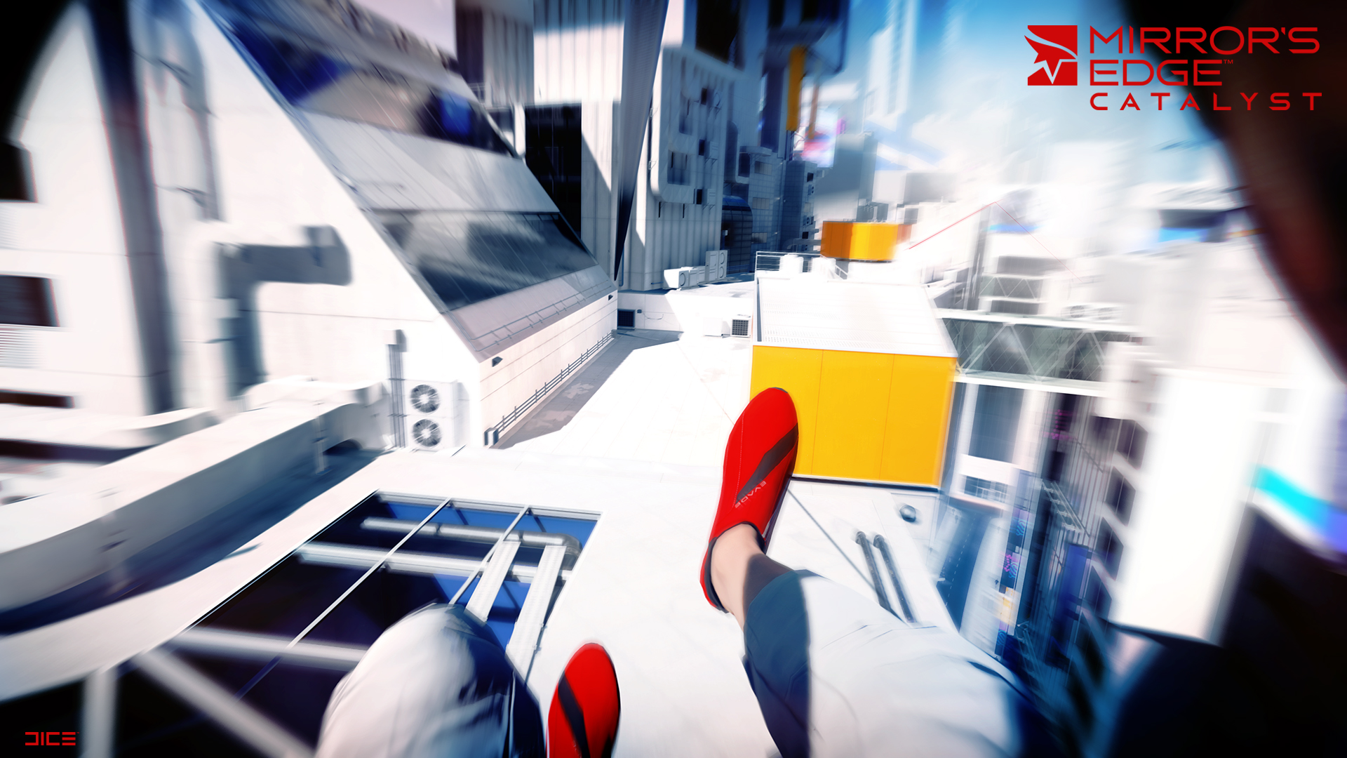
Interactive Illustration 3.17:
A screen shot from a computer game called Mirror's Edge Catalyst by DICE. Note that every object
rendered in this image consists of a set of triangles, where the color of each
pixel inside the triangle has been computed used a short program written by the game developer. To determine
whether a pixel is inside a triangle, the graphics processor often uses three
edge equations (one for each edge of the triangle).
(Copyright 2015 Electronic Arts Inc.)
(Copyright 2015 Electronic Arts Inc.)
3.6.2 Planes
Planes in three dimensions (and higher) are similar to lines in two dimensions in that they both split their domain into two half-spaces. In Section 3.6.1, we saw that a two-dimensional line splits the $xy$-plane into a positive half-space and a negative half-space. There are also two types of representations (one implicit and one explicit) for planes, similar to lines in two dimensions.
To define a plane on explicit form, i.e., similar to $P(t) = S + t\vc{d}$ for lines, a starting point, $S$, and two direction vectors, $\vc{d}_1$ and $\vc{d}_2$, are needed. The direction vectors may not be collinear, i.e., $\vc{d}_1 \neq k \vc{d}_2$ for all values of $k$. Another way to put it is that the direction vectors may not be parallel, not even parallel but with opposite directions. The direction vectors both lie in the plane. Hence, if a point, $P$, is to lie in the plane, it must hold that
| \begin{equation} \overrightarrow{SP} = t_1 \vc{d}_1 + t_2\vc{d}_2, \end{equation} | (3.70) |
| \begin{gather} \overrightarrow{SP(t_1,t_2)} = t_1 \vc{d}_1 + t_2\vc{d}_2 \\ \Longleftrightarrow \\ P(t_1, t_2) - S = t_1 \vc{d}_1 + t_2\vc{d}_2 \\ \Longleftrightarrow \\ P(t_1, t_2) = S + t_1 \vc{d}_1 + t_2\vc{d}_2. \\ \end{gather} | (3.71) |
Definition 3.8:
A Parameterized Plane
A plane, parameterized by $t_1\in\R$ and $t_2\in\R$, can be described by a starting point, $S$, and two direction vectors, $\vc{d}_1$ and $\vc{d}_2$. All points, $P(t_1,t_2)$, on the plane can be described by
If one of $\vc{d}_1$ or $\vc{d}_2$ is $\vc{0}$ or if $\vc{d}_1$ and $\vc{d}_2$ are parallel (either in
the same direction, or opposite), then this degrades to a parameterized line equation.
Interestingly, there is also an implicit form of the plane equation. First, let us write out the plane
equation on component form, as shown below, where $d_{1,y}$ means the $y$-component of $\vc{d}_1$, and so on.
A plane, parameterized by $t_1\in\R$ and $t_2\in\R$, can be described by a starting point, $S$, and two direction vectors, $\vc{d}_1$ and $\vc{d}_2$. All points, $P(t_1,t_2)$, on the plane can be described by
| \begin{equation} P(t_1, t_2) = S + t_1 \vc{d}_1 + t_2\vc{d}_2. \end{equation} | (3.72) |
| \begin{equation} P(t_1, t_2) = S + t_1 \vc{d}_1 + t_2\vc{d}_2 \ \ \ \Longleftrightarrow \ \ \ \begin{cases} p_x(t_1,t_2) = s_x + t_1 d_{1,x} + t_2 d_{2,x},\\ p_y(t_1,t_2) = s_y + t_1 d_{1,y} + t_2 d_{2,y},\\ p_z(t_1,t_2) = s_z + t_1 d_{1,z} + t_2 d_{2,z}. \end{cases} \end{equation} | (3.73) |
| \begin{equation} \vc{n} \cdot (P - S) = 0, \end{equation} | (3.74) |
Definition 3.9:
Implicit Plane Equation
A plane can be represented on implicit form by using a starting point, $S$, and a normal vector, $\vc{n}$. All points, $P$, in the plane can then be described by
Note that $\vc{d}\neq \vc{0}$, otherwise, the expression is always zero.
Exactly as for lines, we can also create a signed distance function as
A plane can be represented on implicit form by using a starting point, $S$, and a normal vector, $\vc{n}$. All points, $P$, in the plane can then be described by
| \begin{equation} \vc{n} \cdot (P - S) = 0. \end{equation} | (3.75) |
| \begin{equation} e(P) = \vc{n} \cdot (P - S), \end{equation} | (3.76) |
Example 3.10:
Orthogonal Projection of a Point onto a Plane
In this example, we will show how a point, $P$, can be projected orthogonally onto a plane defined by a normal, $\vc{n}$, and a starting point, $S$. First, this process is shown in Interactive Illustration 3.19.
The expression for the projected point, $Q$, is simply
where $\vc{v}=P-S$.
Since the projection formula is $\proj{\vc{n}}{\vc{v}} = \bigl( (\vc{v} \cdot \vc{n})/(\ln{\vc{n}}^2) \bigr)\vc{n}$,
i.e., a scalar times $\vc{n}$, we know that $\vc{n}$ is the only vector that is used in creating $Q$ (except for vectors
involved in computing scalar values). Therefore, we know that $Q$ will be projected along a direction orthogonal to the plane.
In fact, since the projection of $\vc{v}$ onto $\vc{n}$ was used to move the point $P$, the point $Q$
must also lie in the plane. However, we can also prove this by entering $Q$ into the plane equation,
i.e., testing whether $\vc{n} \cdot (Q-S)=0$. This is done below.
Note that projecting a point (or vector) to a plane also is similar to computing the reflection vector,
which is the topic of Example 3.13 below.
Next follows an example, where both line equations and plane equations are used.
In this example, we will show how a point, $P$, can be projected orthogonally onto a plane defined by a normal, $\vc{n}$, and a starting point, $S$. First, this process is shown in Interactive Illustration 3.19.
$P$
$S$
$\vc{n}$
$\vc{v}$
$\proj{\vc{n}}{\vc{v}}$
$-\proj{\vc{n}}{\vc{v}}$
$Q$
Interactive Illustration 3.19:
This illustration will show how a point, $P$ (gray circle), is projected orthogonally down
the a plane surface defined by
a normal vector, $\vc{n}$, and a starting point, $S$. The point can be moved around in this illustration.
Click/touch Forward to commence the illustration.
Interactive Illustration 3.19:
This illustration will show how a point, $\hid{P}$ (gray circle), is projected orthogonally down
the a plane surface defined by
a normal vector, $\hid{\vc{n}}$, and a starting point, $\hid{S}$. The point can be moved around in this illustration.
Click/touch Forward to commence the illustration.
| \begin{equation} Q = P - \proj{\vc{n}}{\vc{v}}, \end{equation} | (3.77) |
| \begin{align} \vc{n} \cdot (Q-S) =& \vc{n} \cdot (P - \proj{\vc{n}}{\vc{v}} - S) \\ =& \vc{n} \cdot (\underbrace{P-S}_{\vc{v}} - \proj{\vc{n}}{\vc{v}}) \\ =& \vc{n} \cdot (\vc{v} - \proj{\vc{n}}{\vc{v}}) \\ =& \vc{n} \cdot \vc{v} - \vc{n} \cdot \underbrace{ \Biggl(\frac{\vc{v} \cdot \vc{n}}{\ln{\vc{n}}^2}\vc{n}\Biggr) }_{ \proj{\vc{n}}{\vc{v}} }\\ =& \vc{n} \cdot \vc{v} - \vc{n} \cdot \Biggl(\frac{\vc{v} \cdot \vc{n}}{\ln{\vc{n}}^2}\vc{n}\Biggr)\\ =& \vc{n} \cdot \vc{v} - \frac{\vc{v} \cdot \vc{n}}{\ln{\vc{n}}^2} (\vc{n} \cdot \vc{n})\\ =& \vc{n} \cdot \vc{v} - \frac{\vc{n} \cdot \vc{v}}{\ln{\vc{n}}^2} \ln{\vc{n}}^2 = 0\\ \end{align} | (3.78) |
Example 3.11:
Shadow Projection on a Plane
In this example, we will assume that there is a light source located at $L$, and there is also a triangle with three vertex positions, $V_i$, $i\in \{1,2,3\}$. The triangle will cast a shadow onto a plane, defined by a starting point, $S$, and a normal, $\vc{n}$, i.e., the plane equation is: $\vc{n} \cdot (P-S)=0$ for all points, $P$, lying in the plane. The entire process is illustrated in Interactive Illustration 3.20, and after the reader has explored it, the math will be derived.
To calculate where the shadow "lands" on the plane, we need to create one ray per vertex.
All three rays will start at the light source position, $L$, and the direction per vertex
will be: $\vc{d}_i = V_i - L$, i.e., the ray direction is formed by the line segment created
from the $L$ and $V_i$. Hence, the line equations for the rays will be
Now, what we really are looking for is when these rays "hit" the plane, i.e., we need to set up
an expression which uses the line equations, $R_i(t)$, and the plane equation, $\vc{n}\cdot(P-S)=0$
at the same time. Since the only points, $P$, that lie in the plane fulfill $\vc{n}\cdot(P-S)=0$,
and because we also want those points $P$ to lie on the line equation, we can simply replace
$P$ by $R_i(t)$ in the plane equation and simplify the expression. This is done below.
As can be seen, this is a first-degree polynomial in $t$, which has the following solution (where
we now have added the subscript $i$ to $t$ in order to clearly show that there is one solution
per triangle vertex), i.e.,
Division by zero must be avoided, so let us take a closer look at the denominator, $\vc{n}\cdot\vc{d}_i$,
which is zero only when $\vc{n} \perp \vc{d}_i$, which make sense, because if the ray direction is
parallel to the plane, the ray cannot hit the plane at all. Alternatively, the ray may
lie exactly in the plane, in which case there are an infinite number of solutions.
However, this would mean that the light source would be located in the (ground) plane
as well as the triangle vertex, which is not a situation that is likely to happen (at least in real life).
Anyway, the points of intersection are calculated as $R_i(t_i) = L + t_i\vc{d}_i$. The shadow triangle is then formed from $R_1$, $R_2$, and $R_3$, which is exactly what was done in order to create Interactive Illustration 3.20.
In this example, we will assume that there is a light source located at $L$, and there is also a triangle with three vertex positions, $V_i$, $i\in \{1,2,3\}$. The triangle will cast a shadow onto a plane, defined by a starting point, $S$, and a normal, $\vc{n}$, i.e., the plane equation is: $\vc{n} \cdot (P-S)=0$ for all points, $P$, lying in the plane. The entire process is illustrated in Interactive Illustration 3.20, and after the reader has explored it, the math will be derived.
$L$
$V_1$
$V_2$
$V_3$
$S$
$\vc{n}$
$\vc{d}_1$
$\vc{d}_2$
$\vc{d}_3$
Interactive Illustration 3.20:
This illustration shows how a shadow, projected onto a plane, can be calculated.
Initially, there is a light source (located at $L$), illustrated as a yellow circle,
a triangle with three vertices, $V_i$, and a ground plane. The plane
is described as: $\vc{n}\cdot(P-S)=0$.
Click/touch Forward to commence the illustration.
Interactive Illustration 3.20:
Finally, a shadow triangle is shown.
Note that the light source position can be moved around in this illustration.
Be careful, however, in certain situations, unpredictable illustrations will occur.
Still, it is interesting to move the light source so that it is located under the
triangle. The current calculations still produce a shadow (sometimes called an anti-shadow),
even though this would not be physically correct.
| \begin{equation} R_i(t) = L + t \vc{d}_i, \text{ where } \vc{d}_i = V_i - L, \text{ for } i\in \{1,2,3\}. \end{equation} | (3.79) |
| \begin{equation} \begin{array}{c} \left. \begin{array}{l} R_i(t) = L + t \vc{d}_i \\ \vc{n}\cdot(P-S)=0 \end{array} \right\} \Longrightarrow \vc{n}\cdot(R_i(t)-S) =0 \\ \Longleftrightarrow \\ \vc{n}\cdot(L + t \vc{d}_i-S) = 0 \\ \Longleftrightarrow \\ \vc{n}\cdot (L-S) + t (\vc{n}\cdot\vc{d}_i) = 0 \end{array} \end{equation} | (3.80) |
| \begin{equation} t_i = \frac{-\vc{n}\cdot (L-S)}{\vc{n}\cdot\vc{d}_i} = \frac{\vc{n}\cdot (S-L)}{\vc{n}\cdot\vc{d}_i}. \end{equation} | (3.81) |
Anyway, the points of intersection are calculated as $R_i(t_i) = L + t_i\vc{d}_i$. The shadow triangle is then formed from $R_1$, $R_2$, and $R_3$, which is exactly what was done in order to create Interactive Illustration 3.20.
In the introduction of this chapter (Section 3.1), a graphics program, called a ray tracer, is shown in Interactive Illustration 3.1. Such a program is rather straightforward to write, once some knowledge about linear algebra has been obtained. At the core of a ray tracer, there is a visibility function that determines which object a ray can "see". An example is shown to the right. In a ray tracer, one creates a virtual viewer, which has a position, and is looking in a certain direction. The ray tracer then computes an image from that position in that direction. The view position is the starting point of the blue ray to the right. A set of rays is then created. In the simplest case, one ray per pixel in the image plane is created. It is then up to the ray tracing program to examine the relevant objects in the scene, and compute whether a ray through a pixel hits an object, and also to find the closest object. For the ray in Figure 3.21, we can see that the ray hits two of the three circles. However, since the yellow circle is closer, the pixel is colored yellow. For the pixel above, however, the corresponding ray that goes through that pixel will hit the green circle, and the pixel is therefore colored green. To generate images with shadows, reflections, and refraction, more rays may be shot from the first intersection point between the yellow circle and the ray.
In this section, two examples, which relate to ray tracing, will be shown. The first shows how to compute the intersections between a three-dimensional ray and a three-dimensional sphere. The second example, shows how a vector can be reflected in a surface, whose normal is known. Both of these examples use the dot product as a major tool.
Example 3.12:
Ray-Sphere Intersection
A sphere can be defined by a radius, $r$, and a center point, $C$. The sphere surface is then described as all points, $P$, whose distance from the center, $C$, is equal to the radius, $r$. This can be expressed as
As seen in Section 3.6.1, a three-dimensional line, which we also call a ray here, is
often parameterized
by a parameter, $t$, and it has an origin or starting point, $S$, and a direction, $\vc{d}$.
The ray on explicit form is then (see Definition 3.6)
Now, if $R(t)$ and $P$ are the same, then the ray hits the sphere in that point.
Therefore, we replace $P$ with the ray equation, $R(t)$, and simplify to get
where $a=\vc{d}\cdot\vc{d}$, $b=\vc{d}\cdot(S-C)$, and $c=(S-C)\cdot(S-C)-r^2$.
As can be seen, this turned into a second degree polynomial, which can be solved analytically, i.e.,
Note that if $\vc{d}$ is normalized, i.e., $\ln{\vc{d}}=1$, then $t$ is the distance from the origin, $S$,
along the ray to the intersection point(s) between the sphere and the line segment. However,
it must also hold that $b^2 -ac \geq 0$, otherwise $t$ will become a complex number, and there is
no straightforward interpretation of a imaginary distance $t$ along a ray. Hence, the ray does
not intersect the sphere when $b^2 -ac < 0$. As can be seen, there can be two solutions, $t_1$ and $t_2$,
and these correspond to the entry point and exit point, i.e., the ray first intersects the sphere
in an entry point, and the ray can exit the sphere in another point. These points are computed
as $R(t_1)$ and $R(t_2)$. If $t_1=t_2$ the ray just touches the sphere in a single point.
This is all shown in Interactive Illustration 3.22 below.
A sphere can be defined by a radius, $r$, and a center point, $C$. The sphere surface is then described as all points, $P$, whose distance from the center, $C$, is equal to the radius, $r$. This can be expressed as
| \begin{equation} \ln{P - C} = r. \end{equation} | (3.82) |
| \begin{equation} R(t) = S + t\vc{d}. \end{equation} | (3.83) |
| \begin{gather} \ln{P - C} = r \\ \Longleftrightarrow \\ \ln{S + t\vc{d} - C} = r \\ \Longleftrightarrow \\ (S + t\vc{d} - C) \cdot (S + t\vc{d} - C)= r^2 \\ \Longleftrightarrow \\ t^2(\vc{d}\cdot\vc{d}) + 2t(\vc{d}\cdot(S-C)) + (S-C)\cdot(S-C)-r^2 = 0 \\ \Longleftrightarrow \\ at^2 + 2bt +c =0, \end{gather} | (3.84) |
| \begin{equation} t = \frac{-b \pm \sqrt{b^2 -ac}}{a}. \end{equation} | (3.85) |
$S$
$\vc{d}$
$R(t_1)$
$R(t_2)$
$C$
Interactive Illustration 3.22:
A ray, $R(t) = S + t\vc{d}$ is tested for intersection against a circle.
The ray direction and the circle center can be moved by clicking/touching, pressing and moving around.
As we saw above, the derivation ended up in a second-degree polynomial, which may have at most two
solutions, $t_1$ and $t_2$. These can be used to create two points, $R(t_1)$ and $R(t_2)$, which
are the two points of intersection. The two points (when they exist) are shown as a red and a green filled circle.
The reader is encouraged to explore what happens to the intersection points when the ray origin is
inside the circle, and also attempt to make $R(t_1)$ and $R(t_2)$ come as close as possible to each other.
Interactive Illustration 3.22:
A ray, $\hid{R(t) = S + t\vc{d}}$ is tested for intersection against a circle.
The ray direction and the circle center can be moved by clicking/touching, pressing and moving around.
As we saw above, the derivation ended up in a second-degree polynomial, which may have at most two
solutions, $\hid{t_1}$ and $\hid{t_2}$. These can be used to create two points, $\hid{R(t_1)}$ and $\hid{R(t_2)}$, which
are the two points of intersection. The two points (when they exist) are shown as a red and a green filled circle.
The reader is encouraged to explore what happens to the intersection points when the ray origin is
inside the circle, and also attempt to make $\hid{R(t_1)}$ and $\hid{R(t_2)}$ come as close as possible to each other.
Example 3.13:
Law of Reflection
As seen in the image in the introduction (Section 3.1) of this chapter, the reflected image in a sphere could be computed. To be able to do that, one needs to be able to compute the reflected vector, which can be computed using dot products. We also need the law of reflection, which says that the angle of incidence is equal to the angle of reflection. This is shown for three-dimensional vectors in Interactive Illustration 3.23.
Now that we have seen how the reflected vector (Interactive Illustration 3.23)
is constructed geometrically,
let us see how the reflected vector is expressed mathematically, i.e.,
If $\vc{n}$ is normalized, i.e., $\ln{\vc{n}}=1$, then the above simplifies to
Note that $\vc{r}$ must lie in the same plane as spanned by $\vc{i}$ and $\vc{n}$,
since $2(\vc{i}\cdot\vc{n})$ is a scalar and hence only a scaled version of $\vc{n}$ has been added to $\vc{i}$.
Let us also show that the incident angle is equal to the reflected angle, i.e.,
$[-\vc{i},\vc{n}] = [\vc{r},\vc{n}]$ (note the minus sign on $\vc{i}$, which is needed since $\vc{i}$
points in towards the point, while $\vc{r}$ points away).
For simplicity, let us assume that $\vc{i}$ and $\vc{n}$ are normalized.
This means that $\cos [-\vc{i},\vc{n}] = -\vc{i} \cdot \vc{n}$. The dot product between the reflected
vector, $\vc{r}$, and the normal vector, $\vc{n}$, can be expressed and simplified as below.
As can be seen, the cosine for the incident angle and the reflected angle are the same, and
since only the smallest (and positive) angles between vectors are calculated using
dot products, and because the cosine between $0$ and $\pi$ is unique, then the angles must be the same as well.
This can be proven also for incident and normal vectors of arbitrary lengths. This is, however, left as
an exercise.
As seen in the image in the introduction (Section 3.1) of this chapter, the reflected image in a sphere could be computed. To be able to do that, one needs to be able to compute the reflected vector, which can be computed using dot products. We also need the law of reflection, which says that the angle of incidence is equal to the angle of reflection. This is shown for three-dimensional vectors in Interactive Illustration 3.23.
$\vc{i}$
$\vc{n}$
$\vc{i}$
$\proj{\vc{n}}{\vc{i}}$
$-\proj{\vc{n}}{\vc{i}}$
$-\proj{\vc{n}}{\vc{i}}$
$\vc{r}$
Interactive Illustration 3.23:
This illustration will show how the reflected vector, $\vc{r}$, can be computed, given that we know
the incident vector, $\vc{i}$, and the normal vector, $\vc{n}$, at the hit point.
Here, the incident ray, $\vc{i}$, points towards a gray point.
Click/touch Forward to
commence the illustration.
Interactive Illustration 3.23:
This illustration will show how the reflected vector, $\hid{\vc{r}}$, can be computed, given that we know
the incident vector, $\hid{\vc{i}}$, and the normal vector, $\hid{\vc{n}}$, at the hit point.
Here, the incident ray, $\hid{\vc{i}}$, points towards a gray point.
Click/touch Forward to
commence the illustration.
| \begin{align} \vc{r} =& \vc{i} - \proj{\vc{n}}{\vc{i}} - \proj{\vc{n}}{\vc{i}} \\ =& \vc{i} - 2\proj{\vc{n}}{\vc{i}} \\ =& \vc{i} - 2\frac{\vc{i} \cdot \vc{n}}{\ln{\vc{n}}^2}\vc{n}. \end{align} | (3.86) |
| \begin{equation} \vc{r} = \vc{i} - 2(\vc{i} \cdot \vc{n})\vc{n}. \end{equation} | (3.87) |
| \begin{align} \cos [\vc{r},\vc{n}] =& \vc{r} \cdot \vc{n} \\ =& (\vc{i} - 2(\vc{i} \cdot \vc{n})\vc{n})\cdot \vc{n} \\ =& \vc{i}\cdot \vc{n} - 2(\vc{i} \cdot \vc{n}) \underbrace{(\vc{n}\cdot \vc{n})}_{=1} \\ =& \vc{i}\cdot \vc{n} - 2(\vc{i} \cdot \vc{n}) \\ =& - (\vc{i} \cdot \vc{n}) \end{align} | (3.88) |